
Monday, May 27, 2013 From rOpenSci (https://ropensci.org/blog/2013/05/27/rbison/). Except where otherwise noted, content on this site is licensed under the CC-BY license.
The USGS recently released a way to search for and get species occurrence records for the USA. The service is called BISON (Biodiversity Information Serving Our Nation). The service has a web interface for human interaction in a browser, and two APIs (application programming interface) to allow machines to interact with their database. One of the APIs allows you to search and retrieve data, and the other gives back maps as either a heatmap or a species occurrence map. The latter is more appropriate for working in a browser, so I’ll leave that to the web app folks.
The Core Science Analytics and Synthesis (CSAS) program of the US Geological Survey are responsible for BISON, and are the US node of the Global Biodiversity Information Facility (GBIF). BISON data is nested within that of GBIF, but has (or wil have?) additional data not in GBIF, as described on their About page:
BISON has been initiated with the 110 million records GBIF makes available from the U.S. and is integrating millions more records from other sources each year
Have a look at their Data providers and Statistics tabs on the BISON website, which list where data comes from and how many searches and downloads have been done on each data provider.
We (rOpenSci) started an R package to interact with the BISON search API » rbison. You may be thinking, but if the data in BISON is also in GBIF, why both making another R package for BISON? Good question. As I just said, BISON will have some data GBIF won’t have. Also, the services (search API and map service) are different than those of GBIF.
Check out the package on GitHub here https://github.com/ropensci/rbison.
Here is a quick run through of some things you can do with rbison.
🔗 Install ribson
Install rbison from GitHub using devtools
install.packages('devtools')
library(devtools)
install_github('rbison','ropensci')
library(rbison)
🔗 Search BISON
Do the search
out <- bison(species = "Bison bison", type = "scientific_name", start = 0, count = 10)
Check that the returned object is the right class ‘bison’
class(out)
[1] "bison"
🔗 Summary
bison_data(out)
  total observation fossil specimen unknown
1   761          30      4      709      18
🔗 Summary by counties
Just the first 6 rows
head(bison_data(input = out, datatype = "counties"))
  record_id total county_name      state
1     48295     7    Lipscomb      Texas
2     41025    15      Harney     Oregon
3     49017     8    Garfield       Utah
4     35031     2    McKinley New Mexico
5     56013     1     Fremont    Wyoming
6     40045     2       Ellis   Oklahoma
🔗 Summary of states
bison_data(input = out, datatype = "states")
      record_id total county_fips
1    Washington     1          53
2         Texas     8          48
3    New Mexico     8          35
4          Iowa     1          19
5       Montana     9          30
6       Wyoming   155          56
7        Oregon    15          41
8      Oklahoma    14          40
9        Kansas    10          20
10      Arizona     1          04
11       Alaska    29          02
12         Utah    16          49
13     Colorado    17          08
14     Nebraska     1          31
15 South Dakota    61          46
🔗 Map results
Search for Ursus americanus (american black bear)
out <- bison(species = "Ursus americanus", type = "scientific_name", start = 0,
    count = 200)
Sweet, got some data
bison_data(out)
  total observation fossil specimen literature unknown centroid
1  3792          59    125     3522         47      39       78
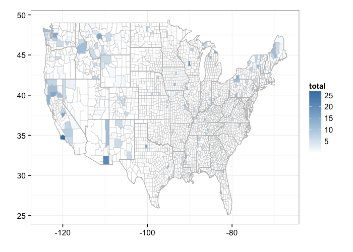
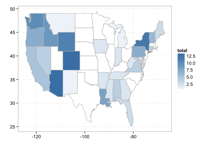
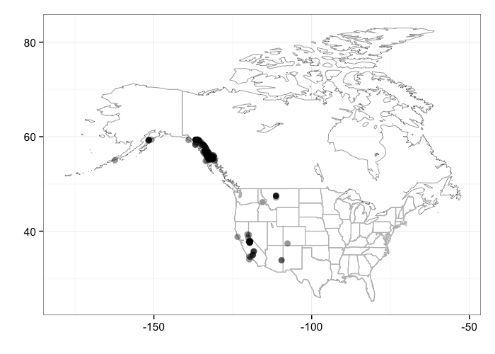
Note that right now the county and state maps just plot the conterminous lower 48. The map of individual occurrences shows the lower 48 + Alaska
By county
bisonmap(out, tomap = "county")
gistr map
By state
bisonmap(out, tomap = "state")
gistr map
Individual locations
bisonmap(out)

gistr map
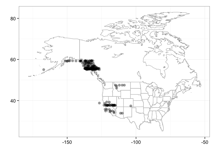
When plotting occurrences, you can pass additional arguments into the bisonmap function. For example, you can jitter the points
bisonmap(input = out, geom = geom_jitter)
gistr map
And you can specify by how much you want the points to jitter (here an extreme example to make it obvious)
library(ggplot2)
bisonmap(input = out, geom = geom_jitter, jitter = position_jitter(width = 5))
gistr map
🔗 Feedback
Let us know if you have any feature requests or find bugs at our GitHub Issues page.
Filed under
Suggest an edit
Open a pull request
