
Tuesday, November 22, 2016 From rOpenSci (https://ropensci.org/blog/2016/11/22/geospatial-suite/). Except where otherwise noted, content on this site is licensed under the CC-BY license.
Geospatial data - data embedded in a spatial context - is used across disciplines, whether it be history, biology, business, tech, public health, etc. Along with community contributors, we’re working on a suite of tools to make working with spatial data in R as easy as possible.
If you’re not familiar with geospatial tools, it’s helpful to see what people do with them in the real world.
Example 1
One of our geospatial packages, geonames, is used for geocoding, the practice of either sorting out place names from geographic data, or vice versa. geonames interfaces with the open database of the same name: https://www.geonames.org/. A recent paper in PlosONE highlights a common use case. Harsch & HilleRisLambers1 asked how plant species distributions have shifted due to climate warming. They used the GNsrtm3() function in geonames, which uses Shuttle Radar Topography Mission elevation data, to fill in missing or incorrect elevation values in their dataset.
Example 2
Another of our packages, geojsonio, is used as a tool to ingest GeoJSON, or make GeoJSON from various inputs. geojsonio was used in Frankfurt’s Open Data Hackathon in March 2016 in a project to present users with random Google Streetview Images of Frankfurt. Check out the repo at safferli/opendataday2016.
We covered the state of our geospatial tools in March of this year, but a lot has changed since then so we thought it would be useful to do an overview of these tools and future work.
There are many geospatial data formats, including shapefiles, GeoTIFF, netCDF, Well-known text/Well-known binary, GeoJSON, and many more. Readers may be more familiar with shape files than WKT or GeoJSON. There are R tools for shape files, so our tools largely don’t concern themselves with shape files and other geospatial data formats. Two formats in particular that we create tools for are GeoJSON and WKT.
🔗 GeoJSON
With the explosion of Javascript/Node and web-first tools, and increasing dominance of JSON as a data format, GeoJSON as a spatial data format has seen increasing use. GeoJSON is a lightweight format based on JSON, and has a very new standard specification: RFC 7946. Many of our geospatial tools center around GeoJSON. Our goal with GeoJSON focused tools is to create a pipeline in which users can process GeoJSON data without any headaches due to dependencies.
- links: specification - Wikipedia entry
- GeoJSON was inspired in part from Simple Features, but is not part of that specification. The most recent iteration is called RFC 7946 GeoJSON.
- Features of note:
- JSON character representation only (though see geobuf for binary GeoJSON - not part of RFC 7946)
- All data is WGS84
- Often found in web applications
🔗 WKT
Well-known text is a plain text format, just like GeoJSON (WKB is a binary form of WKT). It is often used in SQL databases to store geospatial data. Many of the data sources our R packages work with, for example https://www.gbif.org/ (see our package rgbif), use WKT to specify geospatial extent. Thus, rgbif shouldn’t need to import an entire spatial stack that is hard for some to install only for dealing with a single spatial data format - and only some users will do geospatial queries wih WKT as you can constrain queries simply with country names, while others may not need to constrain spatially. We’ve been working on tools to make dealing with WKT more lightweight.
- links: specification - Wikipedia entry
- WKT is part of Simple Features (see
sfbelow) - Features of note:
- Character and binary representations
- Supports any coordinate reference system
- Often used in databases to store geospatial information
🔗 rOpenSci use cases
The motivation for our geospatial tools is supported in part by these use cases for software we make that use WKT and GeoJSON:
- Web services that some of our packages interact with accept a geospatial filter as a query component. This often means WKT. Having tools that are light weight is important here as we don’t need a full geospatial stack when we only need to lint (i.e., validate) WKT or create it from a bounding box, for example.
- Likewise, some web services only accept GeoJSON. Same argument as above applies here.
- Vizualize WKT and GeoJSON: given the above, users should be able to vizualize the area that they are defining with their WKT or GeoJSON.
- WKT-GeoJSON conversion: sometimes one needs to convert WKT to GeoJSON, or vice versa. Light weight tools to do that task are really useful.
🔗 Tools
rOpenSci has a growing suite of database tools:
🔗 GeoJSON/WKT Tools
- geojson (geojson classes for R) (on CRAN)
- geojsonio (I/O for GeoJSON) (on CRAN)
- geojsonlint (Lint GeoJSON) (on CRAN)
- lawn (Turf.js R client) (on CRAN)
- geoaxe (split up well known text into chunks) (on CRAN)
- wellknown (Well-Known-Text <–> GeoJSON) (on CRAN)
- geoops (Operations on GeoJSON, sort of like
rgeos)
🔗 Data/Data Services
- geoparser (Geoparser.io client for place names) (on CRAN)
- rgeospatialquality (spatial quality of biodiversity records) (on CRAN)
- getlandsat (Landsat images) (on CRAN)
- osmplotr (OpenStreeMap data and vizualization) (on CRAN)
- rnaturalearth (Natural Earth data)
- geonames (Access Geonames.org API) (on CRAN)
For each package below, there are 2-3 badges. One for whether the package is on CRAN or not (cran if on CRAN, cran if not), another for link to source on GitHub (github), and another when the package is community contributed (community).
🔗 geojson
We’re excited to announce a new package geojson, which is now on CRAN. Check out the vignettes (geojson classes, geojson operations) to get started.
You can install the package from CRAN:
install.packages("geojson")
library("geojson")
The geojson package has functions for creating each of the GeoJSON classes from character strings of GeoJSON.
feature()- Featurefeaturecollection()- FeatureCollectiongeometrycollection()- GeometryCollectionlinestring()- LineStringmultilinestring()- MultiLineStringmultipoint()- MultiPointmultipolygon()- MultiPolygonpoint()- Pointpolygon()- Polygon
Internally, we perform some basic checks that the string is proper JSON, then if you want to lint
the GeoJSON (see the linting_opts() function) we’ll lint the GeoJSON as well using our
geojsonlint package.
Make a Point
(x <- point('{ "type": "Point", "coordinates": [100.0, 0.0] }'))
#> <Point>
#>   coordinates:  [100,0]
In addition, you can perform some basic operations, such as adding (properties_add()) or getting properties (properties_get()), adding (crs_add()) or getting CRS (crs_get()), adding (bbox_add()) or getting (bbox_get()) a bounding box. You can calculate a bounding box on your GeoJSON with geo_bbox(), prettify your GeoJSON with geo_pretty(), and write your GeoJSON to disk with geo_write().
Add and get properties
(y <- linestring('{ "type": "LineString", "coordinates": [ [100.0, 0.0], [101.0, 1.0] ]}'))
#> <LineString>
#>   coordinates:  [[100,0],[101,1]]
(z <- y %>% feature() %>% properties_add(population = 1000))
#> {
#>     "type": "Feature",
#>     "properties": {
#>         "population": 1000
#>     },
#>     "geometry": {
#>         "type": "LineString",
#>         "coordinates": [
#>             [
#>                 100,
#>                 0
#>             ],
#>             [
#>                 101,
#>                 1
#>             ]
#>         ]
#>     }
#> }
properties_get(z, property = 'population')
#> 1000
Add bbox - without an input, we figure out the 2D bbox for you
x <- '{ "type": "Polygon",
"coordinates": [
  [ [100.0, 0.0], [101.0, 0.0], [101.0, 1.0], [100.0, 1.0], [100.0, 0.0] ]
  ]
}'
y <- polygon(x)
y %>% feature() %>% bbox_add()
#> {
#>     "type": "Feature",
#>     "properties": {
#>
#>     },
#>     "geometry": {
#>         "type": "Polygon",
#>         "coordinates": [
#>             [
#>                 [
#>                     100,
#>                     0
#>                 ],
#>                 [
#>                     101,
#>                     0
#>                 ],
#>                 [
#>                     101,
#>                     1
#>                 ],
#>                 [
#>                     100,
#>                     1
#>                 ],
#>                 [
#>                     100,
#>                     0
#>                 ]
#>             ]
#>         ]
#>     },
#>     "bbox": [
#>         100,
#>         0,
#>         101,
#>         1
#>     ]
#> }
Get the GeoJSON type
geo_type(y)
#> [1] "Polygon"
Pretty print the GeoJSON
geo_pretty(y)
#> {
#>     "type": "Polygon",
#>     "coordinates": [
#>         [
#>             [
#>                 100.0,
#>                 0.0
#>             ],
#>             [
#>                 101.0,
#>                 0.0
#>             ],
#>             [
#>                 101.0,
#>                 1.0
#>             ],
#>             [
#>                 100.0,
#>                 1.0
#>             ],
#>             [
#>                 100.0,
#>                 0.0
#>             ]
#>         ]
#>     ]
#> }
#>
Write to disk (and read back)
f <- tempfile(fileext = ".geojson")
geo_write(y, f)
jsonlite::fromJSON(f, FALSE)
#> $type
#> [1] "Polygon"
#>
#> $coordinates
#> $coordinates[[1]]
#> $coordinates[[1]][[1]]
#> $coordinates[[1]][[1]][[1]]
#> [1] 100
#>
#> $coordinates[[1]][[1]][[2]]
#> [1] 0
#>
#>
#> $coordinates[[1]][[2]]
#> $coordinates[[1]][[2]][[1]]
#> [1] 101
#>
#> $coordinates[[1]][[2]][[2]]
#> [1] 0
#>
#>
#> $coordinates[[1]][[3]]
#> $coordinates[[1]][[3]][[1]]
#> [1] 101
#>
#> $coordinates[[1]][[3]][[2]]
#> [1] 1
#>
#>
#> $coordinates[[1]][[4]]
#> $coordinates[[1]][[4]][[1]]
#> [1] 100
#>
#> $coordinates[[1]][[4]][[2]]
#> [1] 1
#>
#>
#> $coordinates[[1]][[5]]
#> $coordinates[[1]][[5]][[1]]
#> [1] 100
#>
#> $coordinates[[1]][[5]][[2]]
#> [1] 0
Lastly, the Mapbox folks have a compact binary encoding for geographic data (Geobuf) that provides lossless compression of GeoJSON data into protocol buffers. Our own Jeroen Ooms added Geobuf serialization to his protolite package, which we import in geojson to allow you to read Geobuf with from_geobuf() and write Geobuf with to_geobuf().
file <- system.file("examples/test.pb", package = "geojson")
from_geobuf(file, pretty = TRUE)
#> {
#>   "type": "FeatureCollection",
#>   "features": [
#>     {
#>       "type": "Feature",
#>       "geometry": {
#>         "type": "Point",
#>         "coordinates": [102, 0.5]
#>       },
#>       "id": 999,
...
to_geobuf(from_geobuf(file))
#>   [1] 0a 05 70 72 6f 70 30 0a 06 64 6f 75 62 6c 65 0a 0c 6e 65 67 61 74 69
#>  [24] 76 65 5f 69 6e 74 0a 0c 70 6f 73 69 74 69 76 65 5f 69 6e 74 0a 0f 6e
#>  [47] 65 67 61 74 69 76 65 5f 64 6f 75 62 6c 65 0a 0f 70 6f 73 69 74 69 76
#>  [70] 65 5f 64 6f 75 62 6c 65 0a 04 6e 75 6c 6c 0a 05 61 72 72 61 79 0a 06
#>  [93] 6f 62 6a 65 63 74 0a 06 62 6c 61 62 6c 61 0a 07 63 75 73 74 6f 6d 31
...
🔗 geoops
geoops - geoops is not quite ready to use yet, but
the goal with geoops is to provide spatial operations on GeoJSON that work with the geojson
package. Example operations are:
- Find the set of points that are also in a polygon
- Find centroid of a polygon
- Calculate distance between two points
- Calculate buffer of a given radius around a point
- Combine one or more polygons together
Another feature of geoops we’re excited about is slicing up GeoJSON easily by using our
package jqr. It’s similar in concept to using dplyr for drilling down into
a data.frame, but instead we can do that with GeoJSON.
note: this package used to be called
siftgeojson
🔗 geojsonio
geojsonio - geojsonio is a client for making it
easy to convert lots of different things to GeoJSON, and for reading/writing GeoJSON.
We had a new version (v0.2) come out in July this year, with major performance improvements to
geojson_json() - and we’ve deprecated GeoJSON linting functionality and now point people
to our package geojsonlint for all GeoJSON linting tasks.
🔗 Example
A quick example of the power of geojsonio
install.packages("geojsonio")
library("geojsonio")
Convert a numeric vector to a GeoJSON Point:
geojson_json(c(32.45, -99.74))
#> {"type":"FeatureCollection","features":[{"type":"Feature","geometry":{"type":"Point","coordinates":[32.45,-99.74]},"properties":{}}]}
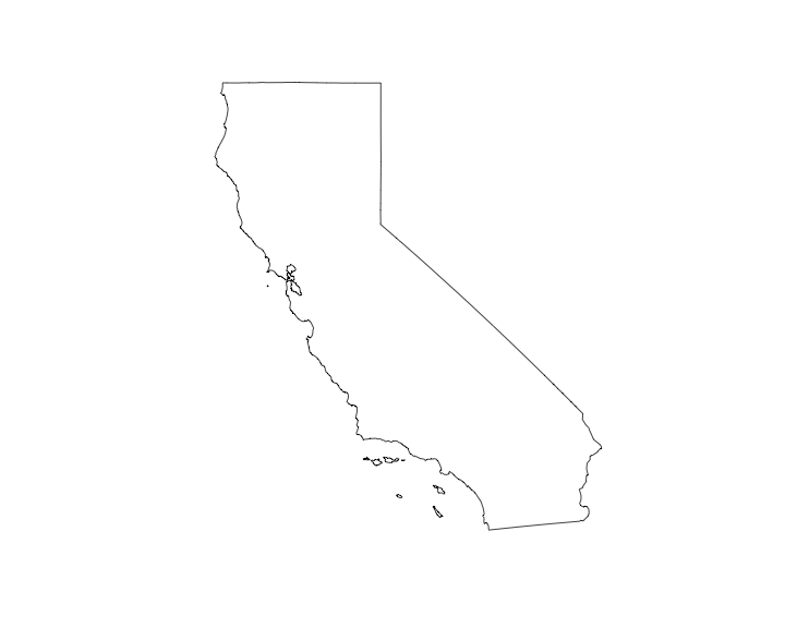
Read GeoJSON from a file with one simple command and plot it:
file <- system.file("examples", "california.geojson", package = "geojsonio")
out <- geojson_read(file, what = "sp")
library('sp')
plot(out)
🔗 geojsonlint
geojsonlint - geojsonlint is a client for linting
GeoJSON. It provides three different ways to lint GeoJSON, using: the API at <geojsonlint.com>,
the JS library geojsonhint, or the JS library is-my-json-valid. The package provides a consistent
interface to the three different linters, always returning a boolean, and toggles provided for
verbose output and whether to stop when invalid GeoJSON is found.
We released a new version (v0.2) this month that uses the newer version of the JS
library geojsonhint, affecting the geojson_hint() function. Note that the dev version of
geojsonlint has an even newer version of the JS geojsonhint library, so you may want to
upgrade if you’re using that linter: devtools::install_github("ropensci/geojsonlint").
🔗 Example
A quick example of the power of geojsonlint
install.packages("geojsonlint")
library("geojsonlint")
Good GeoJSON
geojson_hint(x = '{"type": "Point", "coordinates": [-100, 80]}')
#> [1] TRUE
Bad GeoJSON
geojson_hint('{ "type": "FeatureCollection" }')
#> [1] FALSE
geojson_hint('{ "type": "FeatureCollection" }', verbose = TRUE)
#> [1] FALSE
#> attr(,"errors")
#>   line                    message
#> 1    1 "features" member required
geojson_hint('{ "type": "FeatureCollection" }', error = TRUE)
#> Error: Line 1
#>        - "features" member required
🔗 lawn
lawn - lawn is an R client wrapping Turf.js
from Mapbox. Turf is a JS library for doing advanced geospatial analysis. Using the great V8
R client from Jeroen Ooms we can wrap Turf.js
in R.
We released a new version (v0.3) late last month that is a big change from the previous
version as we now wrap the newest version of Turf v3.5.2 that dropped a number of methods,
and introduced new ones.
🔗 Example
A quick example of the power of lawn
install.packages("lawn")
library("lawn")
Calcuate distance (default: km) between two points
from <- '{
 "type": "Feature",
 "properties": {},
 "geometry": {
   "type": "Point",
   "coordinates": [-75.343, 39.984]
 }
}'
to <- '{
  "type": "Feature",
  "properties": {},
  "geometry": {
    "type": "Point",
    "coordinates": [-75.534, 39.123]
  }
}'
lawn_distance(from, to)
#> [1] 97.15958
Buffer a point (with distance of 5 km)
pt <- '{
 "type": "Feature",
 "properties": {},
 "geometry": {
    "type": "Point",
    "coordinates": [-90.548630, 14.616599]
  }
}'
lawn_buffer(pt, dist = 5)
#> <Feature>
#>   Type: Polygon
#>   Bounding box: -90.6 14.6 -90.5 14.7
#>   No. points: 66
#>   Properties: NULL
🔗 geonames
geonames - geonames is an R client for the
<geonames.org> web service, that allows you to query for global geographic data such
as administrative areas, populated places, and more.
🔗 Example
A quick example of the power of geonames
install.packages("geonames")
library("geonames")
Search for place names with by place name:
GNsearch(q = 'london', maxRows = 10)
#>    adminCode1       lng geonameId             toponymName countryId fcl
#> 1         ENG  -0.12574   2643743                  London   2635167   P
#> 2          08 -81.23304   6058560                  London   6251999   P
#> 3         ENG  -0.09184   2643741          City of London   2635167   P
#> 4          05  27.91162   1006984             East London    953987   P
...
Find the ISO country code for a given lat/long:
GNcountryCode(lat = 47.03, lng = 10.2)
#> $languages
#> [1] "de-AT,hr,hu,sl"
#>
#> $distance
#> [1] "0"
#>
#> $countryCode
#> [1] "AT"
#>
#> $countryName
#> [1] "Republic of Austria"
🔗 geoparser
geoparser - geoparser is an interface
to the Geoparser.io API for Identifying and Disambiguating Places Mentioned in Text
🔗 Example
A quick example of the power of geoparser
install.packages("geoparser")
library("geoparser")
In a very simple example, send a small string to get geoparsed:
output <- geoparser_q("I was born in Vannes and I live in Barcelona")
output$results
#> # A tibble: 2 × 11
#>   country confidence      name admin1                                           type geometry.type longitude latitude reference1 reference2
#> *   <chr>     <fctr>     <chr>  <chr>                                          <chr>        <fctr>     <dbl>    <dbl>      <dbl>      <dbl>
#> 1      FR          1    Vannes     A2 seat of a second-order administrative division         Point  -2.75000 47.66667         14         20
#> 2      ES          1 Barcelona     56  seat of a first-order administrative division         Point   2.15899 41.38879         35         44
#> # ... with 1 more variables: text_md5 <chr>
output$properties
#> # A tibble: 1 × 4
#>   apiVersion       source                    id                         text_md5
#> *     <fctr>       <fctr>                <fctr>                            <chr>
#> 1      0.4.1 geoparser.io 7Mp287nh6XbbH0QMojB6L 51e05aeb3366e55795a9729dd74ae901
The properties data.frame gives some metadata for your request, while the
results data.frame gives results of the geoparsing, including the
name found, the type of geospatial thing, geometry type, and coordinates.
🔗 rgeospatialquality
rgeospatialquality - rgeospatialquality
is an R client for the Geospatial Data Quality API
that detects geospatial quality issues with geostpaial biodiversity occurrence data.
🔗 Example
A quick example of the power of rgeospatialquality
install.packages("rgeospatialquality")
library("rgeospatialquality")
Make a simple occurrence record:
rec <- list(
  decimalLatitude = 42.1833,
  decimalLongitude = -1.8332,
  countryCode = "ES",
  scientificName = "Puma concolor"
)
Pass the record to the API:
parse_record(record = rec)
#> $hasCoordinates
#> [1] TRUE
#>
#> $validCountry
#> [1] TRUE
#>
#> $validCoordinates
#> [1] TRUE
#>
#> $hasCountry
#> [1] TRUE
#>
#> $coordinatesInsideCountry
#> [1] TRUE
#>
#> $hasScientificName
#> [1] TRUE
#>
#> $highPrecisionCoordinates
#> [1] TRUE
#>
#> $coordinatesInsideRangeMap
#> [1] FALSE
#>
#> $nonZeroCoordinates
#> [1] TRUE
#>
#> $distanceToRangeMapInKm
#> [1] 6874.023
The results is a named list, with results for various aspects of geospatial quality, including whether the record has coordinates, whether the country is valid, whether the coordinates are valid, and more.
🔗 getlandsat
getlandsat - getlandsat provides
access to Landsat https://landsat.usgs.gov 8 metadata and images hosted on
AWS S3 at https://aws.amazon.com/public-data-sets/landsat. The package only
fetches data. It does not attempt to aid users in downstream usage.
🔗 Example
A quick example of the power of getlandsat
install.packages("getlandsat")
library("getlandsat")
Get an image (see lsat_list(), lsat_scenes(), lsat_scene_files() to find/search
for images):
lsat_image("LC80101172015002LGN00_B5.TIF")
#> [1] "/Users/sacmac/Library/Caches/landsat-pds/L8/010/117/LC80101172015002LGN00/LC80101172015002LGN00_B5.TIF"
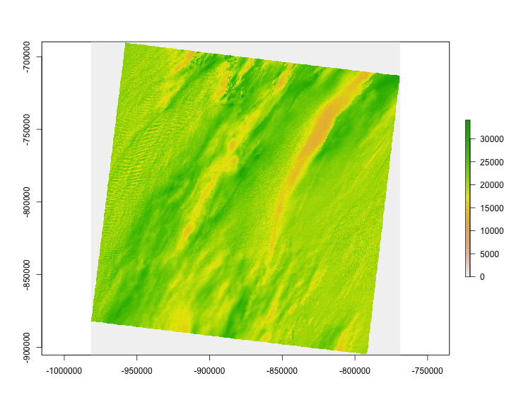
Make a plot
library("raster")
x <- lsat_cache_details()[[1]]
img <- raster(x$file)
plot(img)
🔗 osmplotr
osmplotr - osmplotr produces customisable
images of OpenStreetMap (OSM) data and enables data
visualisation using OSM objects.
🔗 Example
A quick example of the power of osmplotr
install.packages("osmplotr")
library("osmplotr")
library("maptools")
Make a basic map:
bbox <- get_bbox(latlon = c(-0.13,51.50,-0.11,51.52))
dat_B <- extract_osm_objects(key = 'building', bbox = bbox)
map <- osm_basemap(bbox = bbox, bg = 'gray20')
map <- add_osm_objects(map, dat_B, col = 'gray40')
print_osm_map(map)

🔗 rnaturalearth
rnaturalearth - rnaturalearth
facilitates world mapping by making Natural Earth (https://www.naturalearthdata.com/)
map data available in R.
🔗 Example
A quick example of the power of rnaturalearth
devtools::install_github("ropenscilabs/rnaturalearth")
library("rnaturalearth")
Some data comes installed with rnaturalearth
sp::plot(ne_countries())
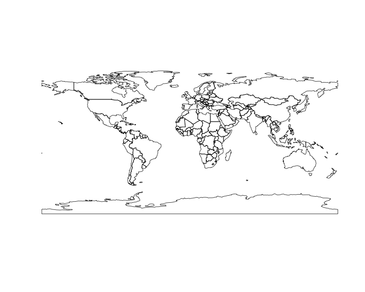
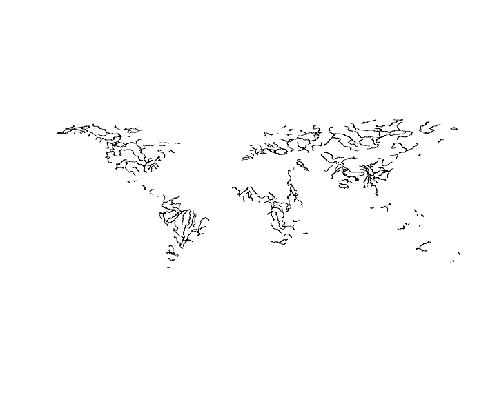
You can also download specific data:
rivers50 <- ne_download(scale = 50, type = 'rivers_lake_centerlines',
                        category = 'physical')
#> OGR data source with driver: ESRI Shapefile
#> Source: "/var/folders/gs/4khph0xs0436gmd2gdnwsg080000gn/T//Rtmp8yl7Kj", layer: "ne_50m_rivers_lake_centerlines"
#> with 460 features
#> It has 4 fields
sp::plot(rivers50)
🔗 Future/Ongoing work
We still have a lot that we’d like to do. Here’s a run down of some of the items on our list:
geoopsfirst version: We need to getgeoopsto a first stable version on CRAN. It will likely be a few months before that happens, as we’re experimenting with how to achieve the best performance, whether that be viajqror dropping down to C/C++.geojson- We just released the first version - We’ll be integratinggeojsoninto some of our other packages that deal with GeoJSON, and may hit upon some improvements we can make togeojson.wellknownfixes: We’re working on our next version of this package, see milestone v0.2, which includes making sure we account for 3D/4D WKT (issue #18), among other things, and there’s a possibility of changing the package interface to be slightly more intuitive (issue #17).geojsonio: milestone v0.3 has a number of bug fixes, and includes methods integrating the new sf package.geojsonrewind: The new GeoJSON specification now has a rule about polygons following a right-hand rule. We’re porting some of Mapbox’s JS stuff to R in geojsonrewind package to be help users fix winding order.
🔗 Takeaway and Feedback
Our goal with our geospatial suite is to make your work – whether it be serious reproducible science, analysis of your company’s data, or just fooling around with some data – as easy as possible with as few installation headaches as possible.
How are you using our geospatial tools? We’d love to hear about how you’re using our packages, whether it be in blog posts, scholarly papers, shiny apps, business use cases, etc.
Let us know if you have any feedback on these packages, and/or if you think there’s anything else we should be thinking about making in this space.
🔗 Community contributors
We’re so so grateful to our community for their hard work on these packages:
- Maëlle Salmon -
geoparser - Andy Teucher -
geojsonio,geojsonlint - Jeff Hollister -
lawn - Mark Padgham -
osmplotr - Andy South -
rnaturalearth - Javier Otegui -
rgeospatialquality - Barry Rowlingson -
geonames
Harsch, M. A., & HilleRisLambers, J. (2016). Climate Warming and Seasonal Precipitation Change Interact to Limit Species Distribution Shifts across Western North America. PLoS ONE, 11(7), e0159184. https://doi.org/10.1371/journal.pone.0159184 ↩︎
Filed under
Suggest an edit
Open a pull request
