
Tuesday, March 7, 2017 From rOpenSci (https://ropensci.org/blog/2017/03/07/hddtools/). Except where otherwise noted, content on this site is licensed under the CC-BY license.
I’ve worked for over 12 years in hydrology and natural hazard modelling and one of the things that still fascinates me is the variety of factors that come into play in trying to predict phenomena such as river floods. From local observations of meteorological and hydrological variables and their spatio-temporal patterns to the type and condition of soils and vegetation/land use as well as the geometry and state of river channels and engineering structures affecting the flow.
This large number of well known predictors directly translates in the need to collect a wide variety of information such as in-situ sensor observations, river survey data, satellite imagery and, more recently, social media information (reporting in real-time the evolution of on-going events). In this field, data collection is challenging on many levels: data are available from different providers under a variety of licences, in various data types and formats that need to be handled and homogenised.
On the one side, not much can be done to overcome licensing issues and the learning curve to become an expert hydrologist is rather steep. On the other side, the R community is working hard to provide tools to make data standards more user-friendly and the convenience of data APIs available to everyone, not only web developers. Here is where hddtools comes into play! This R package is a proof of concept that hydrological data can be made more accessible and consists of a collection of functions to retrieve and homogenise hydrological information. Let me walk you through the main functionalities!
🔗
The R package hddtools
The name hddtools stands for Hydrological Data Discovery Tools. This is an open source project designed to facilitate access to on-line data sources. This typically implies the download of a metadata catalogue, selection of information needed, formal request for dataset(s), de-compression, conversion, manual filtering and parsing. All those operation are made more efficient by re-usable functions.
Depending on the data license, functions can provide offline and/or on-line modes. When redistribution is allowed, for instance, a copy of the dataset is cached within the package and updated twice a year. This is the fastest option and also allows offline use of functions. When re-distribution is not allowed, only on-line mode is provided.
🔗 Installation
The hddtools package and the examples in this blog depend on other CRAN packages. Before attempting to install hddtools, solve any missing dependencies using the commands below:
packs <- c("zoo", "sp", "RCurl", "XML", "rnrfa", "Hmisc", "raster",
           "stringr", "devtools", "leaflet")
new_packages <- packs[!(packs %in% installed.packages()[,"Package"])]
if(length(new_packages)) install.packages(new_packages)
The package is available from the Comprehensive R Archive Network (CRAN):
install.packages("hddtools")
However, the development of this package is very dynamic. Data sources become often unavailable or migrate to new systems. URLs change and, as a consequence, functions may stop working. For this reason, I always suggest to use the development version of this package, which is available from github using devtools:
devtools::install_github("ropensci/hddtools")
Load the hddtools package:
library("hddtools")
🔗 Data sources and Functions
In my quest for hydrological data I found that there are tons of open datasets available but the problem is that you need to know where to look!
Here is the list of data sources available within the hddtools package:
- The Koppen Climate Classification map
- The Global Runoff Data Centre
- NASA’s Tropical Rainfall Measuring Mission
- The Top-Down modelling Working Group:
- Data60UK
- MOPEX -SEPA river level data
For each source, functions are available to obtain and/or filter relevant data. Their usage is described below.
🔗 The Koppen Climate Classification map
The Koppen Climate Classification is the most widely used system for classifying the world’s climates. Its categories are based on the annual and monthly averages of temperature and precipitation. This climate classification is used, in hydrological studies, to explain the continental-scale variability in
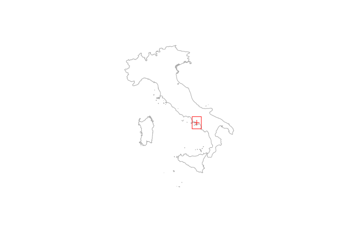
annual runoff. The hddtools package contains a function to identify the updated Koppen-Greiger climate zone, given a bounding box. In the example below I’m getting the climate class for my beautiful home town in Italy: Pompeii.
Country borders are retrieved using the getData() function from the raster package, which retrieves global administrative areas from the following website: http://www.gadm.org/.
# Plot Pompeii on a map
library(raster)
Italy <- getData("GADM", country = "IT", level = 0)
Pompeii <- SpatialPoints(coords = data.frame(x = 14.4870, y = 40.7510))
plot(Italy, col = NA, border = "darkgrey")
plot(Pompeii, add = TRUE, col = "red")

# Define and plot a bounding box centred in Pompeii (Italy)
areaBox <- raster::extent(Pompeii@coords[[1]] - 0.5, Pompeii@coords[[1]] + 0.5,
                          Pompeii@coords[[2]] - 0.5, Pompeii@coords[[2]] + 0.5)
plot(areaBox, add = TRUE, col = "red")
# Extract climate zones from Kottek's map:
KGClimateClass(areaBox = areaBox, updatedBy = "Kottek")
##   ID Class Frequency
## 1 34   Csa       131
From the column Class in the above table, it can be derived that the area falls in a warm temperate climate (C) with dry (s) and hot summers (a). A description of the retrieved class and related criterion can be printed setting the argument verbose = TRUE in the function KGClimateClass().
🔗 The Global Runoff Data Centre
The Global Runoff Data Centre (GRDC) is an international archive hosted by the Federal Institute of Hydrology in Koblenz, Germany. The Centre operates under the auspices of the World Meteorological Organisation and retains services and datasets for all the major rivers in the world. The data catalogue, kml files and the Long-Term Mean Monthly Discharges are open data and accessible via hddtools.
Information on all the GRDC stations can be retrieved using the function catalogueGRDC with no input arguments, as in the example below:
# GRDC full catalogue
GRDC_catalogue_all <- catalogueGRDC()
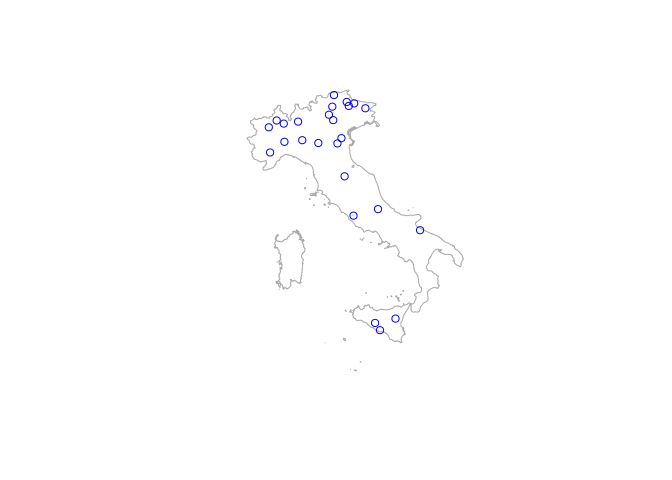
However, there are a number of options to filter the catalogue and return only a subset of stations. For instance, the catalogue can be filtered based on a geographical bounding box as in the function KGClimateClass(). It might also be interesting to subset only stations in a given country, e.g. Italy. As the 8th column in the catalogue lists the country codes, the catalogue can be filtered passing two input arguments to the catalogueGRDC() function: columnName = "country_code" and columnValue = "IT", as in the example below.
# Filter GRDC catalogue based on a country code
GRDC_IT <- catalogueGRDC(columnName = "country_code", columnValue = "IT")

# Convert the table to a SpatialPointsDataFrame
hydro <- SpatialPointsDataFrame(coords = GRDC_IT[, c("long", "lat")],
                                data = GRDC_IT)

# Plot the stations on the map
plot(Italy, col = NA, border = "darkgrey")
plot(hydro, add = TRUE, col = "blue", pch = 1)
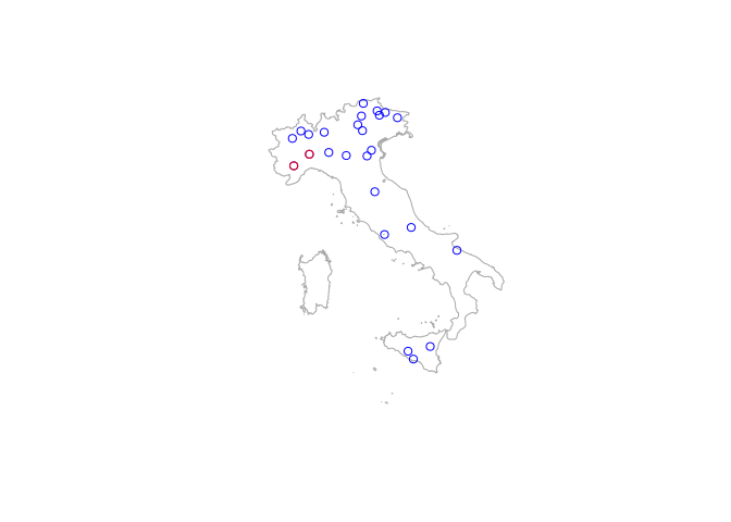
The arguments columnName and columnValue can be used to filter over other columns. For instance, the example below shows how to subset stations along the Tanaro River which source in the Ligurian Alps.
# Filter GRDC catalogue based on rivername, search is not case sensitive!
Tanaro <- catalogueGRDC(columnName = "river", columnValue = "Tanaro")

# Convert the table to a SpatialPointsDataFrame
TanaroSP <- SpatialPointsDataFrame(coords = Tanaro[, c("long", "lat")],
                                   data = Tanaro)

# Highight in red the stations on the Tanaro River
plot(Italy, col = NA, border = "darkgrey")
plot(hydro, add = TRUE, col = "blue", pch = 1)
plot(TanaroSP, add = TRUE, col = "red", pch = 1)
If columnName refers to a numeric field, in the columnValue other terms of comparison can be specified. For example, it is straightforward to find out that the country with the most longstanding monitoring stations is Germany (with 11 out of 15 stations with more than 150 years of recordings).
# Filter GRDC stations with more than 150 years of recordings
GRDC150 <- catalogueGRDC(columnName = "d_yrs", columnValue = ">150")

# Which country has the most longstanding monitoring stations?
table(GRDC150$country_code)
##
## DE FI LT RO SE
## 11  1  1  1  1
# Where is the oldest station?
oldest <- GRDC150[which(GRDC150$d_yrs == max(GRDC150$d_yrs)),
                  c("grdc_no", "river", "station", "d_yrs")]
oldest
## # A tibble: 1 × 4
##   grdc_no      river station d_yrs
##     <chr>      <chr>   <chr> <dbl>
## 1 6340120 ELBE RIVER DRESDEN   208
The oldest stastion is in Dresden on the Elbe River. Let’s now find out whether monthly data is available. For this we need the GRDC identification number (this is stored in the column grdc_no of the catalogue) and the function tsGRDC().
# Monthly data extraction
DresdenStation <- tsGRDC(stationID = oldest$grdc_no, plotOption = TRUE)
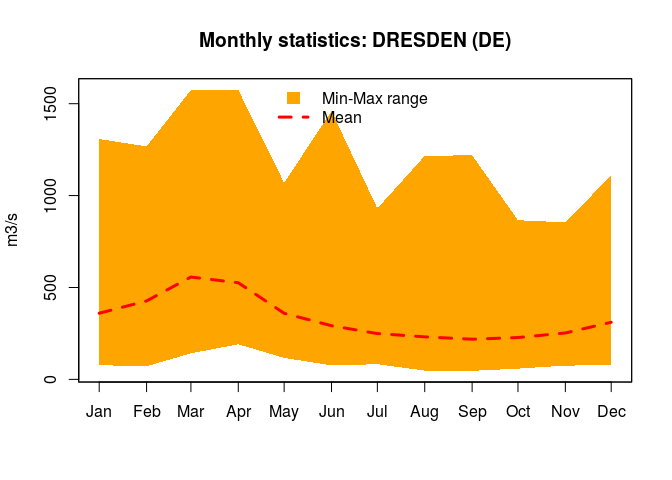
The plot above, shows the time on the x-axis and the flow (in m3/s) on the y-axis. The river flow has had huge oscillations over time, is this an effect of anthropogenic changes and/or climate change? This is well out of the scope of this blog post, I leave the reader to look at trends from the mean monthly values DresdenStation$mddPerYear.
🔗 NASA’s Tropical Rainfall Measuring Mission
The Tropical Rainfall Measuring Mission (TRMM) is a joint mission between NASA and the Japan Aerospace Exploration Agency (JAXA) that uses a research satellite to measure precipitation within the tropics in order to improve our understanding of climate and its variability.
The TRMM satellite records global historical rainfall estimation in a gridded format since 1998 with a daily temporal resolution and a spatial resolution of 0.25 degrees (spatial extent goes from -50 to +50 degrees latitude). This information is openly available for educational purposes and downloadable from an FTP server. The hddtools provides a function, called TRMM(), to download and convert a selected portion of the TRMM dataset into a raster-brick that can be opened in any GIS software.
As an example, I’m going to download precipitation maps for three months in 2016 using the areabox defined previously to locate Pompeii and surrounding areas. But remember, values become less reliable moving away from the tropics!
# Define a temporal extent
twindow <- seq(as.Date("2016-01-01"), as.Date("2016-03-31"), by = "months")

# Retrieve mean monthly precipitations based on a bounding box and time extent
TRMMfile <- TRMM(twindow = twindow, areaBox = areaBox)

plot(TRMMfile)
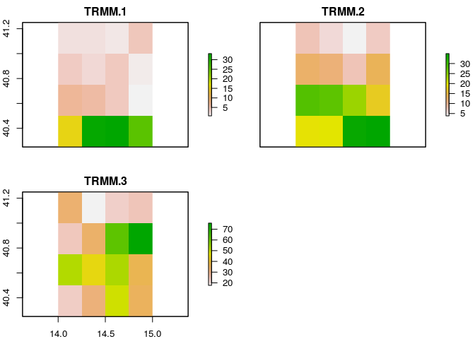
Each of the above plots shows the average precipitation over Pompeii during January (top left), February (top right) and March (bottom left) 2016. Precipitation seems generally more abundant in the south (coastal areas) where the plots show prevalence of green, especially during January and February.
🔗 Top-Down modelling Working Group
The Top-Down modelling Working Group (TDWG) for the Prediction in Ungauged Basins (PUB) Decade (2003-2012) is an initiative of the International Association of Hydrological Sciences (IAHS) which collected datasets for hydrological modelling free-of-charge, available here. This package provides a common interface to retrieve, browse and filter two datasets: Data60UK and MOPEX.
🔗 The Data60UK dataset
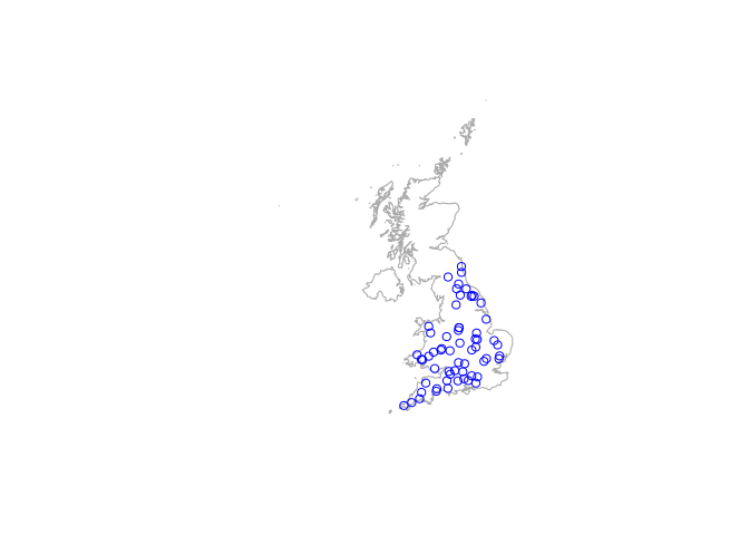
The Data60UK initiative collated datasets of areal precipitation and streamflow discharge across 61 gauging sites in England and Wales (UK). The database was prepared from source databases for research purposes, with the intention to make it re-usable. This is now available in the public domain free of charge.
The hddtools contain two functions to interact with this database: one to retrieve the catalogue and another to retrieve time series of areal precipitation and streamflow discharge.
UK <- getData("GADM", country = "GBR", level = 0)
plot(UK, col = NA, border = "darkgrey")

# Data60UK full catalogue
allData60UK <- catalogueData60UK()
hydroALL <- SpatialPointsDataFrame(coords = allData60UK[, c("Longitude",
                                                         "Latitude")],
                                data = allData60UK)
plot(hydroALL, add = TRUE, col = "blue", pch = 1)
head(allData60UK)
##   stationID        River          Location gridReference Latitude
## 1     22001       Coquet           Morwick      NU234044 55.33310
## 2     22006        Blyth   Hartford Bridge      NZ242800 55.11381
## 3     23006   South Tyne      Featherstone      NY672610 54.94257
## 4     24004 Bedburn Beck           Bedburn      NZ117321 54.68382
## 5     25005        Leven      Leven Bridge      NZ444120 54.50139
## 6     25006        Greta Rutherford Bridge      NZ033122 54.50511
##   Longitude
## 1 -1.632691
## 2 -1.622163
## 3 -2.513539
## 4 -1.820046
## 5 -1.315911
## 6 -1.950550
Given the station identification number (in the column stationID), time series of areal precipitation and streamflow discharge can be downloaded using the function tsData60UK(). In the example below I show how to get the time series for the first station in the table, for a given temporal window.
# Extract time series for the first station
stationID <- catalogueData60UK()$stationID[1]

# Extract time series for a specified temporal window
twindow <- seq(as.Date("1988-01-01"), as.Date("1989-12-31"), by = "days")
MorwickTSplot <- tsData60UK(stationID = stationID,
                            plotOption = TRUE,
                            twindow = twindow)
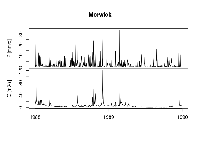
The above figure is divided into two plots: precipitation over time (top) and river flow over time (bottom). High flows and related precipitation events seem to be clearly identifiable. The baseflow is around 10 m3/s, but during the most important events the flow reached 120 m3/s. The shape of the hydrograph, however, suggests that the flow was contained by the embankments and did not cause floods.
🔗 MOPEX
This source contains historical hydrometeorological data and river basin characteristics for hundreds of river basins and from a range of climates in the US. As with the previous dataset, hddtools contains functions to download the catalogue and time series. The example below shows how to download the MOPEX catalogue and the time series for the first station in the catalogue.
# MOPEX full catalogue
allMOPEX <- catalogueMOPEX()

# Extract time series
BroadRiver <- tsMOPEX(stationID = allMOPEX$stationID[1],
                      plotOption = TRUE)
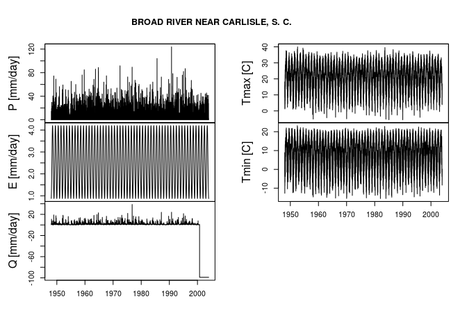
In the plots above P stands for precipitation, E for potential evapotranspiration, Q for river flow, Tmin for minimum temperature and Tmax for maximum temperature.
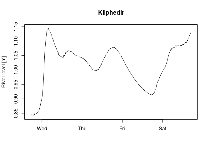
🔗 SEPA river level data
The Scottish Environment Protection Agency (SEPA) manages river level data for hundreds of gauging stations in the UK. The catalogue of stations was derived from a list that’s no longer available, but there’s an equivalent dataset of river levels from the SEPA. The time series of the last few days is available from the SEPA website and can be downloaded using the following function tsSEPA(), as in the example below. Plese note that this data is updated every 15 minutes and the code will always generate different plots.
# SEPA unofficial catalogue
allSEPA <- catalogueSEPA()

# Single time series extraction
Kilphedir <- tsSEPA(stationID = catalogueSEPA()$stationId[1],
                    plotOption = TRUE)
🔗 Example applications
There are a number of possible research applications for the hddtools
package. Retrieved precipitation and streamflow data could, for
instance, be used to draw spatial trends, as done by (Vitolo et al.,
2016b) using the rnrfa package but over larger areas. The package
could also be used to compare hydrological behaviours in different areas
of the world, to run and calibrate hydrological models such as fuse
(Clark et al., 2008, Vitolo et al. 2016a) as well as to undertake
regionalisation studies.
🔗 Future developments
If you have suggestions, please add them to the issue tracker on github. Also, feel free to contribute to the package sending a pull request, that would be greatly appreciated!
🔗 Acknowledgments
I’m very grateful to Erin Le Dell and
Michael Sumner who reviewed, on behalf of
rOpenSci, the hddtools package and the related paper published in the
Journal of Open Source Software (Vitolo, 2017). Both reviewers provided
very constructive suggestions that grately improved this package. I’d
like to also thank Stefanie
Butland and Scott
Chamberlain for providing invaluable advice
when reviewing this post.
🔗 References
Clark, M. P., Slater, A. G., Rupp, D. E., Woods, R. A., Vrugt, J. A., Gupta, H. V., Wagener, T. and Hay, L. E.: Framework for understanding structural errors (fuse): A modular framework to diagnose differences between hydrological models, Water Resources Research, 44(12), n/a–n/a, doi:10.1029/2007WR006735, 2008.
Vitolo, C.: Hddtools: Hydrological data discovery tools, The Journal of Open Source Software, 2(9), doi:10.21105/joss.00056, 2017.
Vitolo, C., Wells, P., Dobias, M. and Buytaert, W.: fuse: An R package for ensemble Hydrological Modelling, The Journal of Open Source Software, 1(8), doi:10.21105/joss.00052, 2016a.
Vitolo, C., Fry, M. and Buytaert, W.: rnrfa: An R package to Retrieve, Filter and Visualize Data from the UK National River Flow Archive, The R Journal, 8(2) [online] Available from: https://journal.r-project.org/archive/2016-2/vitolo-fry-buytaert.pdf, 2016b.
Filed under
Suggest an edit
Open a pull request
