OA week - A simple use case for programmatic access to PLOS full text

doi:https://doi.org/10.59350/w4jr7-pmt65

Tuesday, October 22, 2013 From rOpenSci (https://ropensci.org/blog/2013/10/22/oaweek-rplos/). Except where otherwise noted, content on this site is licensed under the CC-BY license.

OA week - A simple use case for programmatic access to PLOS full text

By Scott Chamberlain

Open access week is here! We love open access, and think it’s extremely important to publish in open access journals. One of the many benefits of open access literature is that we likely can use the text of articles in OA journals for many things, including text-mining.

What’s even more awesome is some OA publishers provide API (application programming interface) access to their full text articles. Public Library of Science (PLOS) is one of these. We have had an R package for a while now that makes it convenient to search PLOS full text programatically. You can search on specific parts of articles (e.g., just in titles, or just in results sections), and you can return specific parts of articles (e.g., just abstracts). There are additional options for more fine-grained control over searches like facetting.

What if you want to find similar papers based on their text content? This can be done using the PLOS search API, with help from the tm R package. These are basic examples just to demonstrate that you can quickly go from a search of PLOS data to a visualization or analysis.

🔗 Install rplos and other packages from CRAN

install.packages(c("rplos", "tm", "wordcloud", "RColorBrewer", "proxy", "plyr"))

🔗 Get some text

library(rplos)
out <- searchplos("birds", fields = "id,introduction", limit = 20, toquery = list("cross_published_journal_key:PLoSONE",
    "doc_type:full"))
out$idshort <- sapply(out$id, function(x) strsplit(x, "\\.")[[1]][length(strsplit(x,
    "\\.")[[1]])], USE.NAMES = FALSE)

The result is a list of length limit defined in the previous call.

nrow(out)

[1] 20

🔗 Word dictionaries

Next, we’ll use the tm package to create word dictionaries for each paper.

library(tm)
library(proxy)
corpus <- Corpus(DataframeSource(out["introduction"]))

# Clean up corpus
corpus <- tm_map(corpus, function(x) removeWords(x, stopwords("english")))
corpus <- tm_map(corpus, function(x) removePunctuation(x))
tdm <- TermDocumentMatrix(corpus)
tdm$dimnames$Docs <- out$idshort

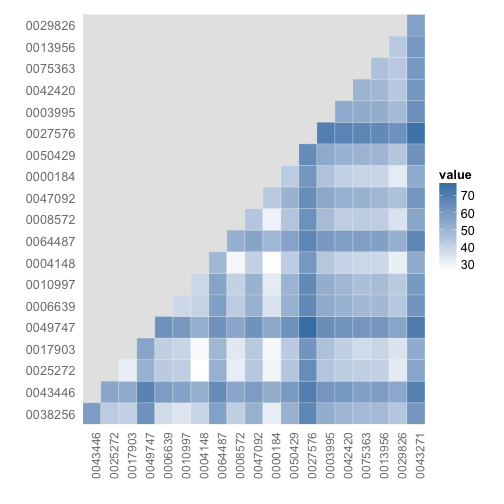
# Comparison among documents in a heatmap
dissmat <- dissimilarity(tdm, method = "Euclidean")
get_dist_frame <- function(x) {
    temp <- data.frame(subset(data.frame(expand.grid(dimnames(as.matrix(x))),
        expand.grid(lower.tri(as.matrix(x)))), Var1.1 == "TRUE")[, -3], as.vector(x))
    names(temp) <- c("one", "two", "value")
    tempout <- temp[!temp[, 1] == temp[, 2], ]
    tempout
}
dissmatdf <- get_dist_frame(dissmat)
ggplot(dissmatdf, aes(one, two)) + geom_tile(aes(fill = value), colour = "white",
    binwidth = 3) + scale_fill_gradient(low = "white", high = "steelblue") +
    theme_grey(base_size = 16) + labs(x = "", y = "") + scale_x_discrete(expand = c(0,
    0)) + scale_y_discrete(expand = c(0, 0)) + theme(axis.ticks = theme_blank(),
    axis.text.x = element_text(size = 12, hjust = 0.6, colour = "grey50", angle = 90),
    panel.grid.major = theme_blank(), panel.grid.minor = theme_blank(), panel.border = theme_blank())

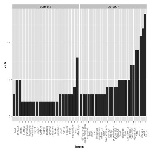
Picking two with low values (=high similarity), dois 10.1371/journal.pone.0000184 and 10.1371/journal.pone.0004148, here’s some of the most common terms used (some overlap).

library(plyr)
df1 <- sort(termFreq(corpus[[grep("10.1371/journal.pone.0010997", out$id)]]))
df1 <- data.frame(terms = names(df1[df1 > 2]), vals = df1[df1 > 2], row.names = NULL)
df2 <- sort(termFreq(corpus[[grep("10.1371/journal.pone.0004148", out$id)]]))
df2 <- data.frame(terms = names(df2[df2 > 1]), vals = df2[df2 > 1], row.names = NULL)
df1$terms <- reorder(df1$terms, df1$vals)
df2$terms <- reorder(df2$terms, df2$vals)
dfboth <- ldply(list(`0010997` = df1, `0004148` = df2))
ggplot(dfboth, aes(x = terms, y = vals)) + geom_histogram(stat = "identity") +
    facet_grid(. ~ .id, scales = "free") + theme(axis.text.x = element_text(angle = 90))

🔗 Determine similarity among papers

Using a wordcloud

library(wordcloud)
library(RColorBrewer)

m <- as.matrix(tdm)
v <- sort(rowSums(m), decreasing = TRUE)
d <- data.frame(word = names(v), freq = v)
pal <- brewer.pal(9, "Blues")
pal <- pal[-(1:2)]

# Plot the chart
wordcloud(d$word, d$freq, scale = c(3, 0.1), min.freq = 2, max.words = 250,
    random.order = FALSE, rot.per = 0.2, colors = pal)