
Wednesday, March 26, 2014 From rOpenSci (https://ropensci.org/blog/2014/03/26/rinat/). Except where otherwise noted, content on this site is licensed under the CC-BY license.
The iNaturalist project is a really cool way to both engage people in citizen science and collect species occurrence data. The premise is pretty simple, users download an app for their smartphone, and then can easily geo reference any specimen they see, uploading it to the iNaturalist website. It let’s users turn casual observations into meaningful crowdsourced species occurrence data. They also provide a nice robust API to access almost all of their data. We’ve developed a package rinat that can easily access all of that data in R. Our package spocc uses iNaturalist data as one of it’s sources, rinat provides an interface for all the features available in the API.
Searching
Currently you can get access to iNaturalist occurrence records from our package spocc, which works great for scenarios where you want lot’s of data from many sources, but rinat will get you full details on every record and offers other searching on terms other than species names. First let’s see how this matches with what you can get with spocc.
options(stringsAsFactors = F)
library(spocc)
## Loading required package: ggplot2
library(rinat)
out <- occ(query = "Accipiter striatus", from = "inat")
inat_out <- get_inat_obs(taxon = "Accipiter striatus", maxresults = 25)
### Compare Id's and see that results are the same without viewing full tables
cbind(out$inat$data$Accipiter_striatus$Id[1:5], inat_out$Id[1:5])
##        [,1]   [,2]
## [1,] 581369 581369
## [2,] 574433 574433
## [3,] 570635 570635
## [4,] 555214 555214
## [5,] 551405 551405
The results are the same, the rinat package will offer a bit more flexiblity in searching. You can search for records by a fuzzy search query, a taxon (used above in spocc), a location in a bounding box, or by date. Let’s say you just want to search by for records of Mayflies, you can use the taxon parameter to search for all lower level taxonomic matches below order.
may_flies <- get_inat_obs(taxon = "Ephemeroptera")
## See what species names come back.
may_flies$Species.guess[1:10]
##  [1] "Mayfly"               "Heptageniidae"        "Ephemerella subvaria"
##  [4] "Ephemerella subvaria" "Mayflies"             "Stream Mayflies"
##  [7] "Mayflies"             "Mayflies"             "Mayflies"
## [10] "Hexagenia"
You could also search using the fuzzy query parameter, looking for mentions of a specific habitat or a common name. Below I’ll search for one of my favorite habitats, vernal ponds and see what species come back. Also we can search for common names and see the scientific names (which should be all the same).
vp_obs <- get_inat_obs(query = "vernal pool")
vp_obs$Species.guess[1:10]
##  [1] "Docks (Genus Rumex)"
##  [2] "Blennosperma bakeri"
##  [3] "Rails, Gallinules, and Coots"
##  [4] "Western Spadefoot"
##  [5] "Western Spadefoot"
##  [6] "Eupsilia"
##  [7] "upland chorus frog"
##  [8] "Wood Frog"
##  [9] "Striped Meadowhawk (Sympetrum pallipes)"
## [10] "Ambystoma maculatum"
# Now le'ts look up by common name:

deer <- get_inat_obs(query = "Mule Deer")
deer$Scientific.name[1:10]
##  [1] "Odocoileus hemionus" "Odocoileus hemionus" "Odocoileus hemionus"
##  [4] "Odocoileus hemionus" "Odocoileus hemionus" "Odocoileus hemionus"
##  [7] "Odocoileus hemionus" "Odocoileus hemionus" "Odocoileus"
## [10] "Odocoileus hemionus"
All of these general searching functions return a dataframe that is m x 32 (where m is the requested number of results). The column names are mostly self-explanatory, including, common names, species names, observer id’s, observer names, data quality, licenses and url’s for images so you can go look at the photo a user took.
Filtering
All searches can also be filtered by space and time. You can search for records within a specific bounding box, or on a specific date (but not a range). We can redo our deer search using a bounding box for the western United States.
bounds <- c(38.44047, -125, 40.86652, -121.837)
deer <- get_inat_obs(query = "Mule Deer", bounds = bounds)
cat(paste("The number of records found in your bunding box:", dim(deer)[1],
    sep = " "))
## The number of records found in your bunding box: 47
By checking the dimensions, we can see only 47 records were found. We could try the samething for a given day, month or year. Let’s try searhing for cumulative totals of observations of Ephemeroptera and see if we can detect seasonality.
library(ggplot2)
out <- rep(NA, 12)
for (i in 1:12) {
    out[i] <- dim(get_inat_obs(taxon = "Ephemeroptera", month = i, maxresults = 200))[1]
}
out <- data.frame(out)
out$month <- factor(month.name, levels = month.name)
ggplot(out, aes(x = month, y = out, group = 1)) + geom_point() + stat_smooth(se = FALSE) +
    xlab("Month") + ylab("Cumulative of Mayfly observations") + theme_bw(16)
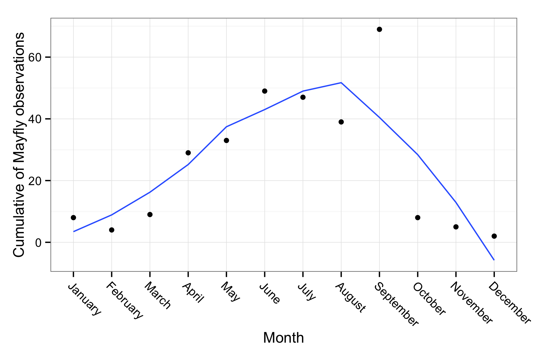
Exactly as you’d expect observations of this season insect tend to peak in the summer and then slowly decline. Except for September peak, it follows the expected trend.
User and project data
There are several other functions from the API that allow you to access data about projects and users. You can grab detailed data about projects, users and observations. Let’s look at the EOL state flowers project. First we can grab some basic info on the project by searching for it based on it’s “slug”.
Let’s grab some info on the project by getting observations but set the type as “info”
eol_flow <- get_inat_obs_project("state-flowers-of-the-united-states-eol-collection",
    type = "info", raw = FALSE)
## 204  Records
## 0
### See how many taxa there are, and how many counts there have been
cat(paste("The project has observed this many species:", eol_flow$taxa_number,
    sep = " "))
## The project has observed this many species: 20
cat(paste("The project has observed this many occurrences:", eol_flow$taxa_count,
    sep = " "))
## The project has observed this many occurrences: 204
We can grab all the observations from the project as well just by setting the type as “observations”. Then it’s easy to to get details about specific observations or users.
eol_obs <- get_inat_obs_project("state-flowers-of-the-united-states-eol-collection",
    type = "observations", raw = FALSE)
## 204  Records
## 0-100-200-300
## See just the first few details of an observation.
head(get_inat_obs_id(eol_obs$Id[1]))
## $captive
## NULL
##
## $comments_count
## [1] 0
##
## $community_taxon_id
## [1] 48225
##
## $created_at
## [1] "2013-04-08T15:49:15-07:00"
##
## $delta
## [1] FALSE
##
## $description
## [1] ""
## See the first five species this user has recorded
head(get_inat_obs_user(as.character(eol_obs$User.login[1]), maxresults = 20))[,
    1]
## [1] "Lynx rufus"              "Melanerpes formicivorus"
## [3] "Lontra canadensis"       "Buteo lineatus"
## [5] "Icteridae"               "Pelecanus occidentalis"
There are many more details that you can get, like counts of observations by place ID (extracted from the project or observation, but not well exposed to users), the most common species by date, or by user. There is almost no end to the details you can extract. If you ever wanted to do a case study of a citizen science project, you could get data to answer almost any question you had about the iNaturalist project with rinat.
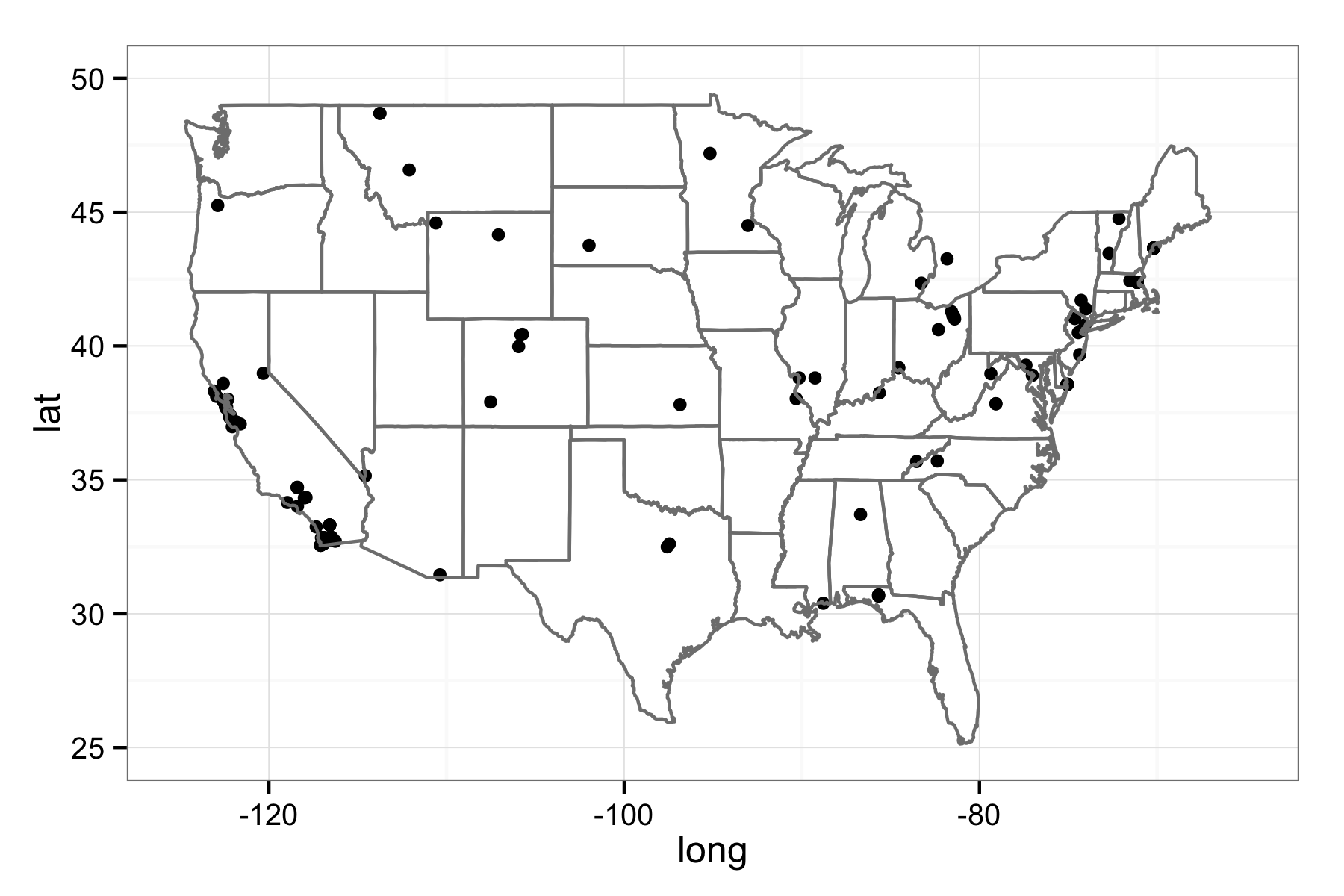
Finally, what species occurrence package wouldn’t be complete without some basic mapping. This function will generate a quick map for you based on a data frame of observations from rinat. These can be from functions such as get_inat_obs, or get_inat_obs_project. Let’s end by plotting all the observations from the EOL state flowers project.
### Set plot to false so it returns a ggplot2 object, and that let's us modify
### it.
eol_map <- inat_map(eol_obs, plot = FALSE)
### Now we can modify the returned map
eol_map + borders("state") + theme_bw() + xlim(-125, -65) + ylim(25, 50)
Filed under
Suggest an edit
Open a pull request
