Monday, November 10, 2014 From rOpenSci (https://ropensci.org/blog/2014/11/10/open-data-growth/). Except where otherwise noted, content on this site is licensed under the CC-BY license.
🔗 Why open data growth
At rOpenSci we try to make it easier for people to use open data and contribute open data to the community. The question often arises: How much open data do we have? Another angle on this topic is: How much is open data growing?
We provide access to dozens of data respositories through our various packages. We asked many of them to share numbers on the amount of data they have, and if possible, growth of their data holdings through time. Many of our partners came through with some data. Note that the below is biased towards those data sources we were able to get data from, and those that we were able to get growth through time data. In addition, note that much of the data we use below was from fall of 2013 (last year) - so the below is based on somewhat old data, but surely the trends are likely still the same now.
We collated data from the different sources, and made some pretty graphs using the data. Here’s what we learned (see last section on how to reproduce this analysis):
🔗 Size of open data
Of the data sources we have data for, how much data is there? The expression of size of data is somewhat different for different sources, so the below is a bit heterogeous, but nonetheless coveys that there is a lot of open data.
rbind(df1, df2) %>%
  mutate(
    type = c('Phenology records','Phylogenetic trees','Taxonomic names','Checklist records','Observations','Taxonomic names','Source databases','Titles','Items','Names','Pages','Species occurrence records','Data publishers','Taxonomic names','Data records','Datasets','Articles','Data packages','SNPs','Users','Genotypes','Data records'),
    source = c('NPN','Treebase','ITIS','eBird','eBird','COL','COL','BHL','BHL','BHL','BHL','GBIF','GBIF','Neotoma','Neotoma','Neotoma','PLOS','Dryad','OpenSNP','OpenSNP','OpenSNP','DataCite')
  ) %>%
  arrange(type, desc(value)) %>%
  kable(format = "html")
| source | value | type |
|---|---|---|
| PLOS | 137358 | Articles |
| eBird | 205970 | Checklist records |
| Dryad | 4186 | Data packages |
| GBIF | 578 | Data publishers |
| DataCite | 3618096 | Data records |
| Neotoma | 2202656 | Data records |
| Neotoma | 11617 | Datasets |
| OpenSNP | 589 | Genotypes |
| BHL | 139561 | Items |
| BHL | 155891133 | Names |
| eBird | 2923886 | Observations |
| BHL | 43968949 | Pages |
| NPN | 2537095 | Phenology records |
| Treebase | 1515 | Phylogenetic trees |
| OpenSNP | 2140939 | SNPs |
| COL | 132 | Source databases |
| GBIF | 420222471 | Species occurrence records |
| COL | 1352112 | Taxonomic names |
| ITIS | 624282 | Taxonomic names |
| Neotoma | 20152 | Taxonomic names |
| BHL | 77258 | Titles |
| OpenSNP | 1230 | Users |
🔗 Growth in open data
First, we have to convert all the date-like fields to proper date classes. The work is not shown - look at the code if you want the details.
🔗 Run down of each data source
🔗 Dryad
- Website: https://datadryad.org/
- R package:
rdryad
Dryad is a repository of datasets associated with published papers. We do have an R package on CRAN (rdryad), but it is waiting on an update for the new API services being built by the Dryad folks. We did recently add in access to their Solr endpoint - check it out.
dryad %>% sort_count %>% gp

gistr map
🔗 OpenSNP
- Website: https://opensnp.org//
- R package:
rsnps
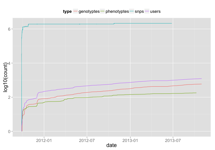
OpenSNP is a collator of SNP datasets that individuals donate to the site/database. They’re an awesome group, and they even won the PLOS/Mendeley code contest a few years back.
opensnp_genotypes <- opensnp_genotypes %>% mutate(type = "genotyptes") %>% sort_count
opensnp_phenotypes <- opensnp_phenotypes %>% mutate(type = "phenotyptes") %>% sort_count
opensnp_snps <- opensnp_snps %>% mutate(type = "snps") %>% sort_count
opensnp_users <- opensnp_users %>% mutate(type = "users") %>% sort_count
os_all <- rbind(opensnp_genotypes, opensnp_phenotypes, opensnp_snps, opensnp_users)
os_all %>%
  ggplot(aes(date, log10(count), color=type)) +
    geom_line() +
    theme_grey(base_size = 18) +
    theme(legend.position = "top")
gistr map
🔗 Datacite
- Website: https://www.datacite.org/
- R package:
rdatacite
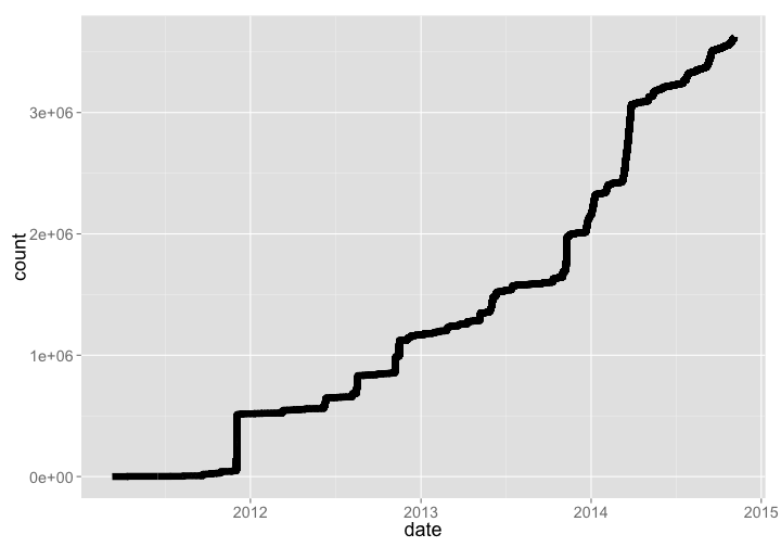
DataCite mints DOIs for datasets, and holds metadata for those datasets provided by data publishers. They have
dcite %>% sort_count %>% gp
gistr map
🔗 US National Phenology Network (USNPN or NPN)
- Website: https://www.usanpn.org/
- R package:
rnpn
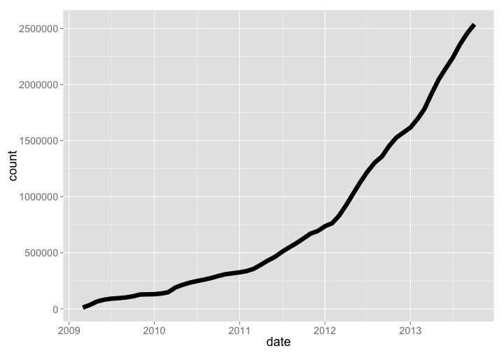
The US National Phenology Network is a project under the USGS. They collect phenology observations across both plants and animals.
npn %>% arrange(date) %>% mutate(count = cumsum(Number_Records)) %>% gp
gistr map
🔗 TreeBASE
- Website: https://treebase.org/
- R package:
treebase
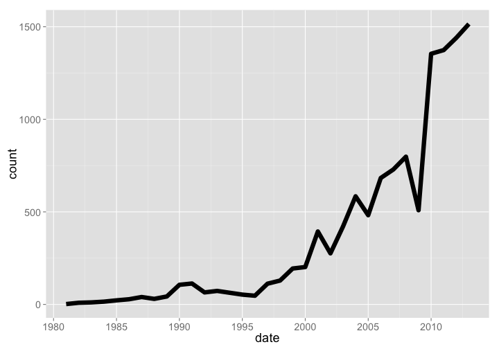
TreeBASE is a database of phylogenetic trees, had a total of 1515 new trees added in 2013, and has been growing at a good pace. Note that these aren’t numbers of total phylogenetic trees, but new trees added each year - we couldn’t get our hands on total number of trees by year. The current number of total trees as of 2015-03-10 is 12,817.
treebase %>% arrange(date) %>% rename(count = New.Trees.Added) %>% gp
gistr map
🔗 Integrated Taxonomic Information Service (ITIS)
- Website: https://www.itis.gov/
- R package:
taxize
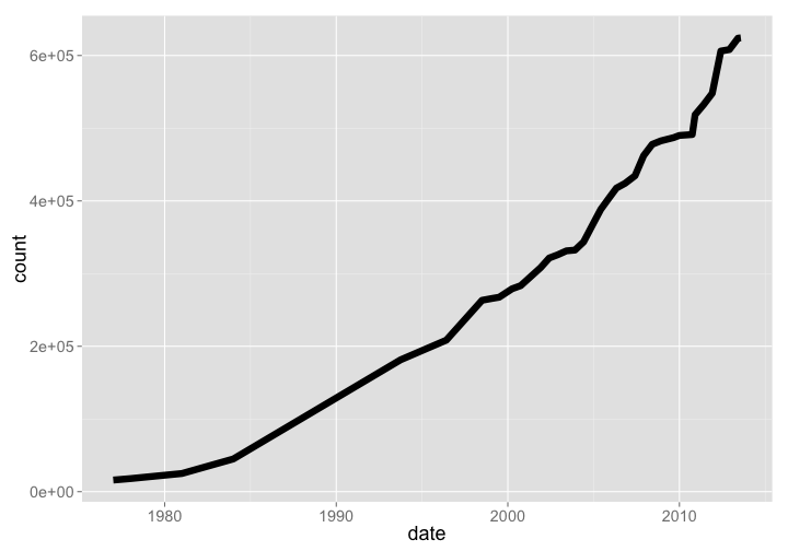
The ITIS database is under the USGS, and holds taxonomic names for mostly North American species. This dataset is interesting, because data goes back to 1977, when they had 16000 names. As of Aug 2013 they had 624282 names.
itis %>% arrange(date) %>% rename(count = total_names) %>% gp
gistr map
🔗 eBird
- Website: https://www.catalogueoflife.org/
- R package:
taxize
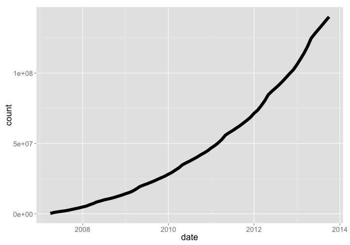
eBird is a database of bird occurence records. They don’t give access to all the data they have, but some recent data. Data growth goes up and down through time because we don’t have access to all data on each data request, but the overall trend is increasing.
ebird_observations %>% arrange(date) %>% mutate(count = cumsum(COUNT.OBS_ID.)) %>% gp
gistr map
🔗 Catalogue of Life (COL)
- Website: https://www.datacite.org/
- R package:
rdatacite
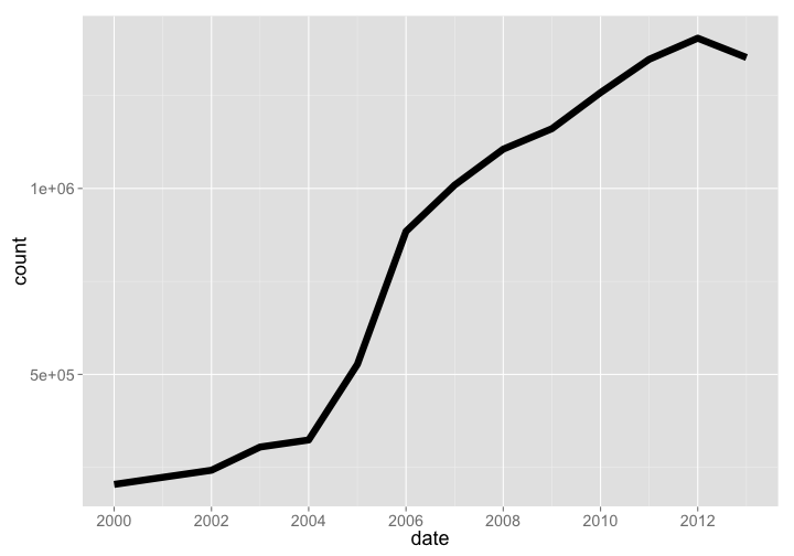
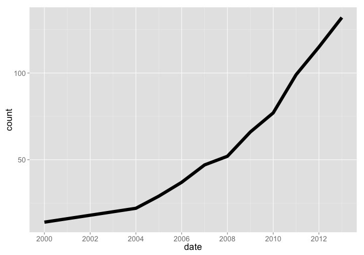
COL is a database of taxonomic names, similar to ITIS, uBio, or Tropicos. The number of species (1352112) has continually increased (the slight level off is because we got data in Oct last year before the year was over), but number of data sources (1352112) was still growing as of 2013.
Number of species
col %>% arrange(date) %>% rename(count = species) %>% gp
gistr map
Number of data sources
col %>% arrange(date) %>% rename(count = source_databases) %>% gp
gistr map
🔗 Public Library of Science (PLOS)
- Website: https://www.plos.org/
- R package:
rplos,fulltext
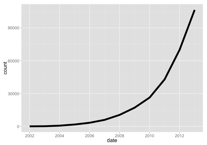
PLOS has had tremendous growth, with a very steep hockey stick growth curve. This year (2014) is left out because the year is not over yet.
plos_years %>%
  arrange(date) %>%
  filter(date < as.Date("2014-01-01")) %>%
  mutate(count = cumsum(articles)) %>%
  gp
gistr map
🔗 Biodiversity Heritage Library (BHL)
- Website: https://www.biodiversitylibrary.org/
- R package:
rbhl
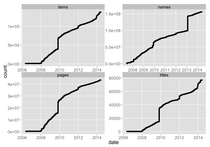
BHL has grown tremendously, with 155891133 names, 43650663 pages, 139003 items, and 77169 titles.
bhl_titles <- bhl_titles %>% mutate(type = "titles") %>% arrange(date) %>% mutate(count = cumsum(Titles))
bhl_items <- bhl_items %>% mutate(type = "items") %>% arrange(date) %>%  mutate(count = cumsum(Items))
bhl_pages <- bhl_pages %>% mutate(type = "pages") %>% arrange(date) %>%  mutate(count = cumsum(Pages))
bhl_names <- bhl_names %>% mutate(type = "names") %>% arrange(date) %>%  mutate(count = cumsum(Names))
bhl_all <- rbind(bhl_titles[,-c(1:4)], bhl_items[,-c(1:4)], bhl_pages[,-c(1:4)], bhl_names[,-c(1:4)])
bhl_all %>%
  ggplot(aes(date, count)) +
    geom_line(size=2.1) +
    theme_grey(base_size = 18) +
    facet_wrap(~ type, scales = "free")
gistr map
🔗 Global Biodiversity Information Facility (GBIF)
- Website: https://www.gbif.org/
- R package:
rgbif,spocc
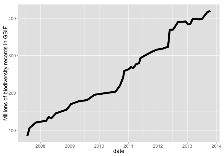
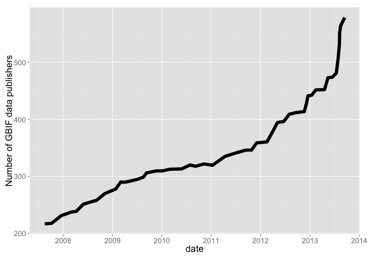
GBIF is the largest warehouse of biodiversity occurrence records, pulling in data from 578, and 420 million occurrence records as of Oct. 2013. Growth through time has been dramatic.
Number of records
gbif_data %>%
  arrange(date) %>%
  rename(count = V2) %>%
  gp + labs(y="Millions of biodiversity records in GBIF")
gistr map
Number of data publishers
gbif_publishers %>%
  arrange(date) %>%
  rename(count = V2) %>%
  gp + labs(y="Number of GBIF data publishers")
gistr map
🔗 Neotoma
- Website: https://www.neotomadb.org/
- R package:
neotoma
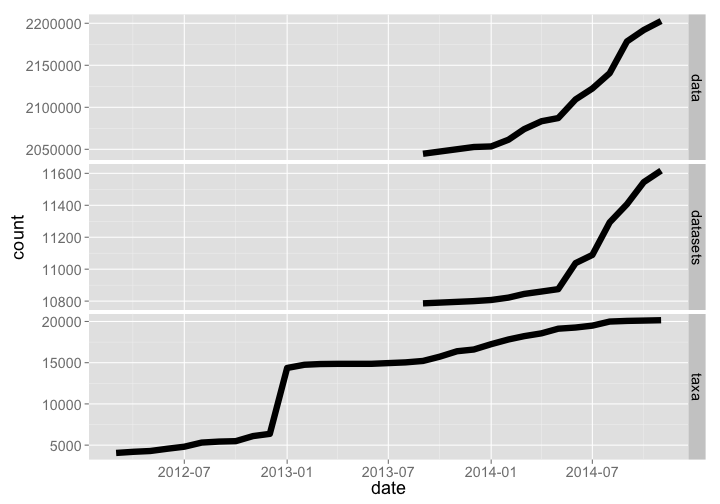
The Neotoma database holds paleoecology records of various kinds, including pollen and fossil records. The R package neotoma allows access to data from Neotoma. Data and datasets have grown rather dramatically, while number of taxa has flattened off recently.
rbind(neotoma_data %>% mutate(type = "data") %>% arrange(date),
      neotoma_datasets %>% mutate(type = "datasets") %>% arrange(date),
      neotoma_taxa %>% mutate(type = "taxa") %>% arrange(date)) %>%
  rename(count = RunningCount) %>%
  gp + facet_grid(type ~ ., scales="free")
gistr map
🔗 So what?
Okay, so a lot of data isn’t that meaningful in itself. But, this is open data that can be used to do science, which means there is an increasingly vast amount of open data as the basis for new research, to supplement field based research, etc. The killer feature of all this open data is that it’s all available programatically through R packages produced in the rOpenSci community, meaning you can easily and quickly do reproducible science with this data.
🔗 Reproduce this analysis
- Option 1: If you are comfortable with git, simply clone the dbgrowth repository to your machine, uncompress the compressed file,
cdto the directory, and runR. Running R should enter packrat mode, which will install packages from within the directory, after which point you can reproduce what we have done above. - Option 2: Install the
packratR package if you don’t have it already. Download this compressed file (a packrat bundle), then in R, runpackrat::unbundle("<path to tar.gz>", "<path to put the contents>"), which will uncompress the file, and install packages, and you’re ready to go.
Once you have the files, you should be able to run knitr::knit("dbgrowth.Rmd") to reproduce this post.

