
Thursday, March 17, 2016 From rOpenSci (https://ropensci.org/blog/2016/03/17/ropensci-geospatial-stack/). Except where otherwise noted, content on this site is licensed under the CC-BY license.
Geospatial data input/output, manipulation, and vizualization are tasks that are common to many disciplines. Thus, we’re keenly interested in making great tools in this space. We have an increasing set of spatial tools, each of which we’ll cover sparingly. See the cran and github badges for more information.
We are not trying to replace the current R geospatial libraries - rather, we’re trying to fill in gaps and create smaller tools to make it easy to plug in just the tools you need to your workflow.
🔗 geojsonio
geojsonio - A tool for converting to and from geojson data. Convert data to/from GeoJSON from various R classes, including vectors, lists, data frames, shape files, and spatial classes.
e.g.
library("geojsonio")
geojson_json(c(-99.74, 32.45), pretty = TRUE)
#> {
#>   "type": "FeatureCollection",
#>   "features": [
#>     {
#>       "type": "Feature",
#>       "geometry": {
#>         "type": "Point",
#>         "coordinates": [-99.74, 32.45]
#>       },
#>       "properties": {}
#>     }
#>   ]
#> }
🔗 wellknown
wellknown - A tool for converting to and from well-known text data. Convert WKT/WKB to GeoJSON and vice versa. Functions included for converting between GeoJSON to WKT/WKB, creating both GeoJSON features, and non-features, creating WKT/WKB from R objects (e.g., lists, data.frames, vectors), and linting WKT.
e.g.
library("wellknown")
point(data.frame(lon = -116.4, lat = 45.2))
#> [1] "POINT (-116.4000000000000057 45.2000000000000028)"
🔗 gistr
gistr - This is not a geospatial tool per se, but it’s extremely useful for sharing maps. For example, with just a few lines, you can share an interactive map to GitHub.
e.g. using geojsonio from above
library("gistr")
cat(geojson_json(us_cities[1:100,], lat = 'lat', lon = 'long'), file = "map.geojson")
gist_create("map.geojson")
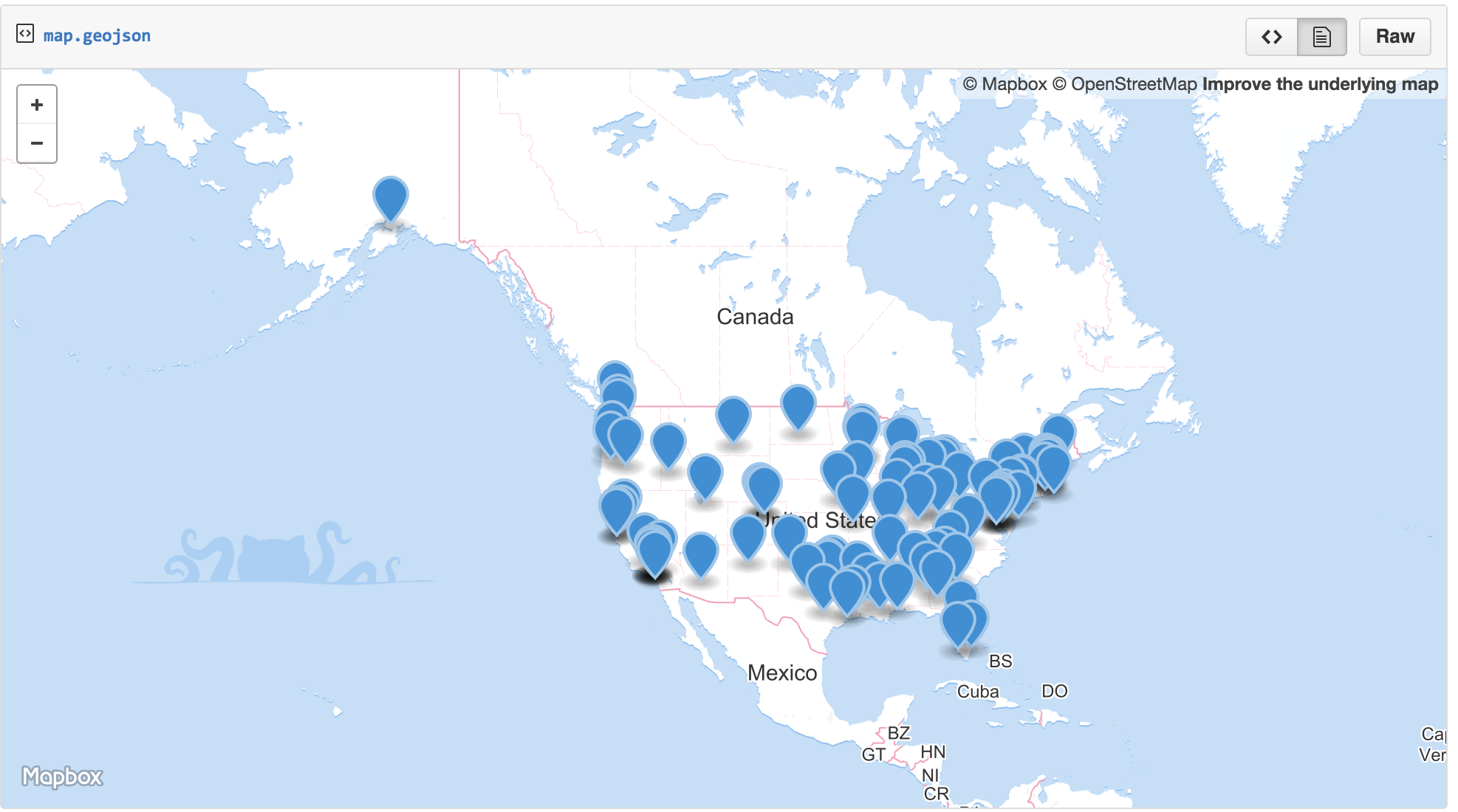
gistr map
🔗 lawn
An R client for turf.js, an Advanced geospatial analysis for browsers and node
lawn has a function for every method in turf.js. In addition, there’s:
- a few functions wrapping the
Node package
geojson-randomhttps://github.com/mapbox/geojson-random for making random geojson features - a helper function
view()to easily visualize results from calls tolawnfunctions
e.g.
library("lawn")
lawn_hex_grid(c(-96,31,-84,40), 50, 'miles') %>% view
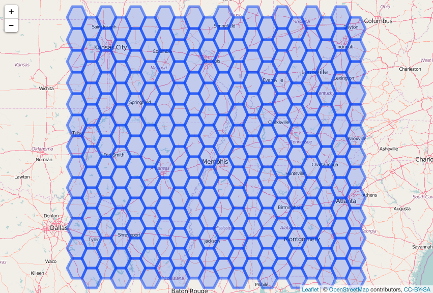
lawn map
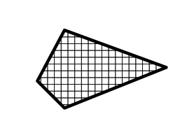
🔗 geoaxe
An R client for splitting geospatial objects into pieces.
e.g.
library("geoaxe")
library("rgeos")
wkt <- "POLYGON((-180 -20, -140 55, 10 0, -140 -60, -180 -20))"
poly <- rgeos::readWKT(wkt)
polys <- chop(x = poly)
plot(poly, lwd = 6, mar = c(0, 0, 0, 0))

geoaxe map
Add chopped up polygon bits
plot(polys, add = TRUE, mar = c(0, 0, 0, 0))
geoaxe map
🔗 proj
An R client for proj4js, a Javascript library for projections. proj is not on CRAN yet.
🔗 getlandsat
An R client to fetch Landsat data from AWS public data sets. getlandsat is not on CRAN yet.
e.g.
library("getlandsat")
head(lsat_scenes())
#>                entityId     acquisitionDate cloudCover processingLevel
#> 1 LC80101172015002LGN00 2015-01-02 15:49:05      80.81            L1GT
#> 2 LC80260392015002LGN00 2015-01-02 16:56:51      90.84            L1GT
#> 3 LC82270742015002LGN00 2015-01-02 13:53:02      83.44            L1GT
#> 4 LC82270732015002LGN00 2015-01-02 13:52:38      52.29             L1T
#> 5 LC82270622015002LGN00 2015-01-02 13:48:14      38.85             L1T
#> 6 LC82111152015002LGN00 2015-01-02 12:30:31      22.93            L1GT
#>   path row   min_lat    min_lon   max_lat    max_lon
#> 1   10 117 -79.09923 -139.66082 -77.75440 -125.09297
#> 2   26  39  29.23106  -97.48576  31.36421  -95.16029
#> 3  227  74 -21.28598  -59.27736 -19.17398  -57.07423
#> 4  227  73 -19.84365  -58.93258 -17.73324  -56.74692
#> 5  227  62  -3.95294  -55.38896  -1.84491  -53.32906
#> 6  211 115 -78.54179  -79.36148 -75.51003  -69.81645
#>                                                                                 download_url
#> 1 https://s3-us-west-2.amazonaws.com/landsat-pds/L8/010/117/LC80101172015002LGN00/index.html
#> 2 https://s3-us-west-2.amazonaws.com/landsat-pds/L8/026/039/LC80260392015002LGN00/index.html
#> 3 https://s3-us-west-2.amazonaws.com/landsat-pds/L8/227/074/LC82270742015002LGN00/index.html
#> 4 https://s3-us-west-2.amazonaws.com/landsat-pds/L8/227/073/LC82270732015002LGN00/index.html
#> 5 https://s3-us-west-2.amazonaws.com/landsat-pds/L8/227/062/LC82270622015002LGN00/index.html
#> 6 https://s3-us-west-2.amazonaws.com/landsat-pds/L8/211/115/LC82111152015002LGN00/index.html
🔗 siftgeojson
Slice and dice GeoJSON just as easily as you would a data.frame. This is built on top of jqr, an R wrapper for jq, a JSON processor.
library("siftgeojson")
# get sample data
file <- system.file("examples", "zillow_or.geojson", package = "siftgeojson")
json <- paste0(readLines(file), collapse = "")
# sift to Multnomah County only, and check that only Multnomah County came back
sifter(json, COUNTY == Multnomah) %>% jqr::index() %>% jqr::dotstr(properties.COUNTY)
#> [
#>     "Multnomah",
#>     "Multnomah",
#>     "Multnomah",
#>     "Multnomah",
#>     "Multnomah",
#>     "Multnomah",
#>     "Multnomah",
#>     "Multnomah",
#>     "Multnomah",
...
🔗 Maps
rOpenSci has an offering in this space: plotly
🔗 plotly
plotly is an R client for Plotly - a web interface and API for creating interactive graphics.
library("plotly")
plot_ly(iris, x = Petal.Length, y = Petal.Width,
        color = Species, mode = "markers")
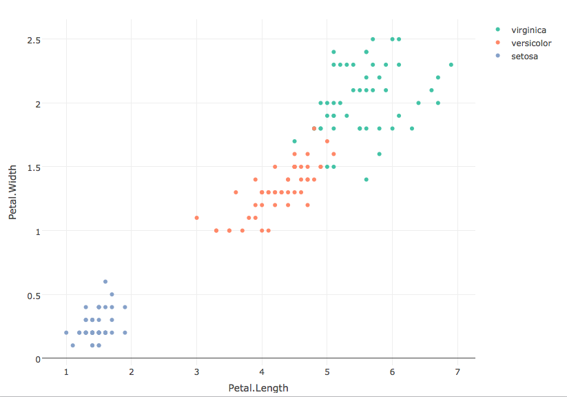
plotly map
🔗 Maptools Task View
Jeff Hollister is leading the maptools task view to organize R mapping tools packages, sources of data, projections, static and interactive mapping, data transformation, and more.
Filed under
Suggest an edit
Open a pull request
