Advanced Image-Processing in R with Magick, Part I

The new magick package is an ambitious effort to modernize and simplify high-quality image processing in R. It wraps the ImageMagick STL which is perhaps the most comprehensive open-source image processing library available today.

The ImageMagick library has an overwhelming amount of functionality. The current version of Magick exposes a decent chunk of it, but being a first release, documentation is still sparse. This post briefly introduces the most important concepts to get started. There will also be an rOpenSci community call on Wednesday in which we demonstrate basic functionality.

🔗 Installation

On Windows or OS-X the package is most easily installed via CRAN.

install.packages("magick")

On Linux you need to install the ImageMagick++ library: on Debian/Ubuntu this is called libmagick++-dev:

sudo apt-get install libmagick++-dev

On Fedora or CentOS/RHEL we need ImageMagick-c++-devel:

sudo yum install ImageMagick-c++-devel

To install from source on OS-X you need imagemagick from homebrew.

brew install imagemagick --with-fontconfig --with-librsvg --with-fftw

The default imagemagick configuration on homebrew disables a bunch of features. I recommend you install --with-fontconfig and --with-librsvg to get high quality font / svg rendering (the CRAN OSX binary package enables these as well).

library(magick)
magick_config()

Use magick_config to see which features and formats are supported by your version of ImageMagick.

🔗 Reading and writing

Images can be read directly from a file path, URL, or raw vector with image data. Similarly we can write images back to disk, or in memory by setting path=NULL.

# Render svg to png
tiger <- image_read('https://upload.wikimedia.org/wikipedia/commons/f/fd/Ghostscript_Tiger.svg')
image_write(tiger, path = "tiger.png", format = "png")

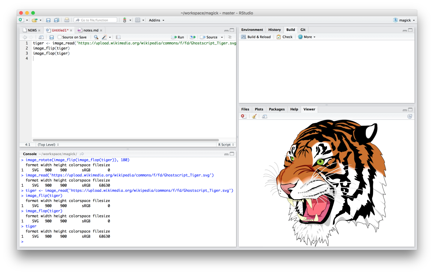
IDE’s with a built-in web browser (such as RStudio) automatically display magick images in the viewer. This results in a neat interactive image editing environment.

Alternatively, on Linux you can use image_display to preview the image in an X11 window. Finally image_browse opens the image in your system’s default application for a given type.

# X11 only
image_display(tiger)

# System dependent
image_browse(tiger)

There is some functionality to convert images to R raster graphics and plot it on R’s graphics display, but this doesn’t always work too well yet.

frink <- image_read("https://jeroen.github.io/images/frink.png")
raster <- as.raster(frink)
plot(raster)

Also the R graphics device is relatively slow for displaying bitmap images.

🔗 Transformations and effects

The best way to get a sense of available transformations is walk through the examples in the ?transformations help page in RStudio. Below a few examples to get a sense of what is possible.

# Example image
frink <- image_read("https://jeroen.github.io/images/frink.png")

# Trim margins
image_trim(frink)

# Passport pica
image_crop(frink, "100x150+50")

# Resize
image_scale(frink, "200x") # width: 200px
image_scale(frink, "x200") # height: 200px

# Rotate or mirror
image_rotate(frink, 45)
image_flip(frink)
image_flop(frink)

# Set a background color
image_background(frink, "pink", flatten = TRUE)

# World-cup outfit (Flood fill)
image_fill(frink, "orange", "+100+200", 30000)

ImageMagick also has a bunch of standard effects that are worth checking out.

# Add randomness
image_blur(frink, 10, 5)
image_noise(frink)

# Silly filters
image_charcoal(frink)
image_oilpaint(frink)
image_emboss(frink)
image_edge(frink)
image_negate(frink)

Finally it can be useful to print some text on top of images:

# Add some text
image_annotate(frink, "I like R!", size = 50)

# Customize text
image_annotate(frink, "CONFIDENTIAL", size = 30, color = "red", boxcolor = "pink",
  degrees = 60, location = "+50+100")

# Only works if ImageMagick has fontconfig
image_annotate(frink, "The quick brown fox", font = 'times-new-roman', size = 30)

Maybe this is enough to get started.

🔗 Layers and animation

The examples above concern single images. However all functions in magick have been vectorized to support working with layers, compositions or animation.

The standard base vector methods [ [[, $, c() and length() are used to manipulate sets of images which can then be treated as layers or frames. This system is actually so extensive that we will do a separate blog post about it later.

For now here is an example on how to generate the instant classic dancing banana on R logo (which is probably why you are here):

# Background image
logo <- image_read("https://www.r-project.org/logo/Rlogo.png")
background <- image_scale(logo, "400")

# Foreground image
banana <- image_read(system.file("banana.gif", package = "magick"))
front <- image_scale(banana, "300")

# Combine and flatten frames
frames <- lapply(as.list(front), function(x) image_flatten(c(background, x)))

# Turn frames into animation
animation <- image_animate(image_join(frames))
print(animation)

# Save as GIF
image_write(animation, "Rlogo-banana.gif")

If time permits we will demonstrate more examples during our community call on Wednesday!