Extracting and Enriching Ocean Biogeographic Information System (OBIS) Data with R

Programmatic access to biodiversity data is revolutionising large-scale, reproducible biodiversity research. In the marine realm, the largest global database of species occurrence records is the Ocean Biogeographic Information System, OBIS. As of January 2017, OBIS contains 47.78 million occurrences of 117,345 species, all openly available and accessible via the OBIS API. The number of questions to address using these kinds of resources is as large as the number of investigators, but certain operations commonly crop up in many workflows. In my group, shefmeme.org, these typically involve checking the taxonomy of a list of species, extracting occurrence records for each species, mapping these and matching them to various environmental and geographic data layers, all using R. I recently wrote up these common operations in a detailed tutorial for OBIS, with associated code and data on GitHub. This tutorial made extensive use of rOpenSci packages and expertise, and so I’m delighted to have the opportunity to present an edited version here. (Please note that the code chunks included here are a subset of our original code, and are for illustration - if you want to run these examples we suggest visiting the original post.)

🔗 Starting point, journey, and destination

We start with a list of taxonomic names of unknown quality. In our experience this is a common situation: you may have obtained a dataset from a collaborator, or from the literature, which documents some characteristics of a number of taxa, and you wish to tidy up this dataset and enrich it with some occurrence data. We generated a taxon list from a museum exhibit in the Department of Animal and Plant Sciences at the University of Sheffield: a collection of 80 marine specimens created by the 19th Century Sheffield microscopist, geologist, and naturalist Henry Clifton Sorby. This provides a useful test-case for modern biodiversity computational methods, as there is considerable taxonomic breadth (including fish as well as numerous invertebrate groups), but the names recorded are of inconsistent taxonomic rank, and - having been recorded well over 100 years ago - many are almost certainly no longer current.

The first stage of our journey then - after transcribing the names into a spreadsheet - is to check their taxonomy. Once we are confident in the names, and have restricted the dataset to a suitable taxonomic rank (species, here), we can start to examine occurrences as recorded in OBIS. Once we have done this, for individual species and for groups of species, we can start to enrich the basic occurrence data in various ways. In particular, we show how to match the occurrences to various environmental layers, including depth and climate. And we show how to perform more sophisticated geographic searches using georeferenced boundaries and regions.

🔗 Taxonomy

OBIS uses the WoRMS standard taxonomy. This means that names within OBIS’s realisation of the WoRMS Aphia database will be matched correctly, but it is still often worthwhile to check your taxonomy in advance, especially if you are working with large sets of taxa (as macroecologists frequently are), or with unusual sets of names, such as the Sorby Collection. This will help to identify any potential problems or ambiguities, and also gives more flexibility for identifying and dealing with minor typos and misspellings. The tools provided by rOpenSci have made it possible to rapidly match names to WoRMS by calling the WoRMS web services directly from within R. In our original post, we provide examples using the taxizesoap package. WoRMS have recently updated their web services, and here we use instead the new rOpenSci package worrms - now incorporated into taxize. Both options provide much of the WoRMS taxon matching functionality, for instance fuzzy (or approximate) name matching is possible, and is a convenient, scripted way of generating a taxonomically robust dataset.

First, load the required libraries:

library(worrms)
library(dplyr)

🔗 Check taxonomy of a single taxon

Get the WoRMS ID for a single species - here, Atlantic cod, Gadus morhua:

my_sp_aphia <- wm_name2id(name = "Gadus morhua")

Then get the full WoRMS record, as a list by Aphia ID:

my_sp_taxo <- wm_record(id = my_sp_aphia)

Or as a tibble by name - here specifying exact match only (fuzzy = FALSE) and restricting to marine species (marine_only = TRUE):

my_sp_taxo <- wm_records_names(name = "Gadus morhua", fuzzy = FALSE, marine_only = TRUE)

🔗 Get taxonomy for multiple species

Start with a data frame of species names:

my_sp <- data_frame(sciname = c("Gadus morhua", "Solea vulgaris", "Pleuronectes platessa"))

Then get the WoRMS records for each:

my_sp_taxo <- wm_records_names(name = my_sp$sciname, fuzzy = FALSE, marine_only = TRUE)

For ’n’ species this returns a list of ’n’ tables. Convert these into a single table with ’n’ rows:

my_sp_taxo <- bind_rows(my_sp_taxo)

And look at the results:

glimpse(my_sp_taxo)

## Observations: 3
## Variables: 25
## $ AphiaID         <int> 126436, 154712, 127143
## $ url             <chr> "https://www.marinespecies.org/aphia.php?p=taxd...
## $ scientificname  <chr> "Gadus morhua", "Solea vulgaris", "Pleuronecte...
## $ authority       <chr> "Linnaeus, 1758", "Quensel, 1806", "Linnaeus, ...
## $ status          <chr> "accepted", "unaccepted", "accepted"
## $ unacceptreason  <chr> NA, "synonym", NA
## $ rank            <chr> "Species", "Species", "Species"
## $ valid_AphiaID   <int> 126436, 127160, 127143
## $ valid_name      <chr> "Gadus morhua", "Solea solea", "Pleuronectes p...
## $ valid_authority <chr> "Linnaeus, 1758", "(Linnaeus, 1758)", "Linnaeu...
## $ kingdom         <chr> "Animalia", "Animalia", "Animalia"
## $ phylum          <chr> "Chordata", "Chordata", "Chordata"
## $ class           <chr> "Actinopteri", "Actinopteri", "Actinopteri"
## $ order           <chr> "Gadiformes", "Pleuronectiformes", "Pleuronect...
## $ family          <chr> "Gadidae", "Soleidae", "Pleuronectidae"
## $ genus           <chr> "Gadus", "Solea", "Pleuronectes"
## $ citation        <chr> "Bailly, N. (2008). Gadus morhua Linnaeus, 175...
## $ lsid            <chr> "urn:lsid:marinespecies.org:taxname:126436", "...
## $ isMarine        <int> 1, 1, 1
## $ isBrackish      <int> 1, 1, 1
## $ isFreshwater    <int> 0, 0, 0
## $ isTerrestrial   <int> 0, 0, 0
## $ isExtinct       <lgl> NA, NA, NA
## $ match_type      <chr> "exact", "exact", "exact"
## $ modified        <chr> "2008-01-15T18:27:08Z", "2008-02-28T14:41:08Z"...

Note that the name we supplied is correct for cod and plaice, but Solea vulgaris is not valid and has the valid name Solea solea.

🔗 Getting occurrences

Once you have your taxon name, or list of names, it is straightforward to extract their OBIS occurrences using the robis package. And armed with a list of occurrences for a given taxon, or list of species, you probably want to map them. Here we show how to obtain and map occurrence records for a single species.

First install and load additional required packages:

# install robis package using devtools
library(devtools)
devtools::install_github("iobis/robis")
# NB - you also need the dev version of ggmap for the satellite maps to work
devtools::install_github("dkahle/ggmap")
library(robis)
library(ggmap)
library(raster)

Get occurrences for sole - note that this may take some time to run:

my_occs <- occurrence(scientificname = my_sp_taxo$valid_name[2])

What is the bounding box for these occurrences?

bb_occs <- bbox(cbind(my_occs$decimalLongitude, my_occs$decimalLatitude))
bb_occs

##        min     max
## x -42.0288 151.639
## y -33.0868  61.250

Get a base world map:

world <- map_data("world")

Create a map from these data:

worldmap <- ggplot(world, aes(x=long, y=lat)) +
  geom_polygon(aes(group=group)) +
  scale_y_continuous(breaks = (-2:2) * 30) +
  scale_x_continuous(breaks = (-4:4) * 45) +
  theme(panel.background = element_rect(fill = "steelblue")) +
  coord_equal()

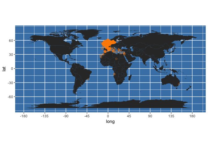
Plot the map and add the occurrence data for sole that we have just returned:

(occ_map <- worldmap + geom_point(data = my_occs, aes(x = decimalLongitude, y = decimalLatitude),
                                 colour = "darkorange", shape = 21, alpha = 2/3)
)

We can wrap this in a function to rapidly plot occurrences returned from OBIS onto a map:

obis_map <- function(occ_dat, map_type = c("satellite", "world"), map_zoom = NULL, plotit = TRUE){

  bb_occ <- bbox(cbind(occ_dat$decimalLongitude, occ_dat$decimalLatitude))

  if(map_type == "satellite"){
    if(is.null(map_zoom)){
      base_map <- get_map(location = bb_occ, maptype = "satellite")
    } else {
      base_map <- get_map(location = bb_occ, maptype = "satellite", zoom = map_zoom)
    }
    obis_map <- ggmap(base_map)
  } else if(map_type == "world"){
    base_map <- map_data("world")
    obis_map <- ggplot(base_map, aes(x=long, y=lat)) +
      geom_polygon(aes(group=group)) +
      scale_y_continuous(breaks = (-2:2) * 30) +
      scale_x_continuous(breaks = (-4:4) * 45) +
      theme(panel.background = element_rect(fill = "steelblue")) +
      coord_equal()
  } else {
    stop("map_type must be one of 'satellite' or 'world'",
         call. = FALSE)
  }

  # Now add the occurrence points
  obis_map <- obis_map + geom_point(data = occ_dat, aes(x = decimalLongitude, y = decimalLatitude),
                                    colour = "darkorange", shape = 21, alpha = 2/3)

  if(plotit == T){print(obis_map)}

  return(obis_map)

}

sole_map <- obis_map(my_occs, map_type = "world", plotit = TRUE)

In our original post we give more examples of plotting records from individual species and multiple species, including gridded richness maps. We also explain the many fields returned by OBIS for each record, and provide examples of filtering results both pre- and post-query on a number of criteria (e.g. date, dataset, and various quality control flags), which can bring important memory savings when the returned set of occurrences is very large.

🔗 Enriching occurrence data

Matching species occurrences to environmental variables is a very common requirement of macroecological analyses, particularly those considering environmental drivers of species distributions, and how distributions are expected to shift as the climate changes. Environmental or geographical data layers of interest may be purely spatial (e.g. bathymetry), or spatio-temporal (e.g. sea surface temperature, SST). In our original post we show how to use the packages robis and marmap (Pante & Simon-Bouhet 2013) to match occurrence records to bathymetry, necessary to perform the kinds of analyses we published here. We also show how to match occurrence records to locally-stored spatial datasets, such as the global marine environmental layers that can be downloaded from GMED. In this post, we focus on obtaining NOAA gridded monthly mean Sea Surface Temperature data and show how to match occurrence records to temperature in both space and time. This code is from a package in development with ROpenSci called spenv, see here, but we use slightly modified versions of spenv functions here.

First, we use a function to download SST data from NOAA. Specifically, it downloads monthly mean data at 1 degree resolution from the Optimum Interpolation Seas Surface Temperature V2 dataset, see here. The data are served as a NetCDF file, but for convenience we transform this into a raster brick - this is essentially a stacked set of global rasters, each layer representing a single month in the time series. The first time you run this the file will be downloaded (takes ~10 seconds). It will then be stored locally for future use.

Start by loading additional required packages:

library(ncdf4)
library(lubridate)

Obtain the SST data from NOAA and convert to raster brick format:

sst_prep <- function(path = "~/.spenv/noaa_sst") {
  x <- file.path(path, "sst.mnmean.nc")
  if (!file.exists(x)) {
    dir.create(dirname(x), recursive = TRUE, showWarnings = FALSE)
    download.file("ftp://ftp.cdc.noaa.gov/Datasets/noaa.oisst.v2/sst.mnmean.nc", destfile = x)
  }
  raster::brick(x, varname = "sst")
}
sst_dat <- sst_prep()

View the structure of the data:

sst_dat

## class       : RasterBrick
## dimensions  : 180, 360, 64800, 417  (nrow, ncol, ncell, nlayers)
## resolution  : 1, 1  (x, y)
## extent      : 0, 360, -90, 90  (xmin, xmax, ymin, ymax)
## coord. ref. : +proj=longlat +datum=WGS84 +ellps=WGS84 +towgs84=0,0,0
## data source : /Users/alunjones/.spenv/noaa_sst/sst.mnmean.nc
## names       : X1981.12.01, X1982.01.01, X1982.02.01, X1982.03.01, X1982.04.01, X1982.05.01, X1982.06.01, X1982.07.01, X1982.08.01, X1982.09.01, X1982.10.01, X1982.11.01, X1982.12.01, X1983.01.01, X1983.02.01, ...
## Date        : 1981-12-01, 2016-08-01 (min, max)
## varname     : sst

Below is a wrapper function that takes your input data (x), together with identifiers for latitude, longitude, and date, and gets SST data from the NOAA SST gridded dataset. The origin argument enables conversion between the date formats of the NOAA data and your occurrence data. Note that this data also calculates an adjusted longitude, as occupancy data typically come with longitude in the range -180 (180 West) to +180 (180 East), whereas the NOAA data codes longitude as 0 to 360 degrees (running eastwards from 0 degrees):

sp_extract_gridded_date <- function(x, from = "noaa_sst", latitude = NULL,
                                    longitude = NULL, samp_date = NULL, origin = as.Date("1800-1-1")) {

  x <- spenv_guess_latlondate(x, latitude, longitude, samp_date)
  switch(from,
         noaa_sst = {
           mb <- sst_prep()
           out <- list()
           x <- x[ !is.na(x$date), ]
           x$date <- as.Date(x$date)
           x <- x[x$date >= min(mb@z[["Date"]]), ]
           x$lon_adj <- x$longitude
           x$lon_adj[x$lon_adj < 0] <- x$lon_adj[x$lon_adj < 0] + 360
           for (i in seq_len(NROW(x))) {
             out[[i]] <- get_env_par_space_x_time(mb, x[i, ], origin = origin)
           }
           x$sst <- unlist(out)
           x
         }
  )
}

You also need these utility functions:

spenv_guess_latlondate <- function(x, lat = NULL, lon = NULL, samp_date = NULL) {
  xnames <- names(x)
  if (is.null(lat) && is.null(lon)) {
    lats <- xnames[grep("^(lat|latitude)$", xnames, ignore.case = TRUE)]
    lngs <- xnames[grep("^(lon|lng|long|longitude)$", xnames, ignore.case = TRUE)]

    if (length(lats) == 1 && length(lngs) == 1) {
      if (length(x) > 2) {
        message("Assuming '", lngs, "' and '", lats,
                "' are longitude and latitude, respectively")
      }
      x <- rename(x, setNames('latitude', eval(lats)))
      x <- rename(x, setNames('longitude', eval(lngs)))
    } else {
      stop("Couldn't infer longitude/latitude columns, please specify with 'lat'/'lon' parameters", call. = FALSE)
    }
  } else {
    message("Using user input '", lon, "' and '", lat,
            "' as longitude and latitude, respectively")
    x <- plyr::rename(x, setNames('latitude', eval(lat)))
    x <- plyr::rename(x, setNames('longitude', eval(lon)))
  }

  if(is.null(samp_date)){
    dates <- xnames[grep("date", xnames, ignore.case = TRUE)]
    if(length(dates) == 1){
      if(length(x) > 2){
        message("Assuming '", dates, "' are sample dates")
      }
      x <- rename(x, setNames('date', eval(dates)))
    } else {
      stop("Couldn't infer sample date column, please specify with 'date' parameter", call. = FALSE)
    }

  } else {
    message("Using user input '", samp_date, "' as sample date")
    x <- plyr::rename(x, setNames('date', eval(samp_date)))
  }

}

And:

get_env_par_space_x_time <- function(
  env_dat, occ_dat, origin = as.Date("1800-1-1")){

  # calculate starting julian day for each month in env_dat
  month_intervals <- as.numeric(env_dat@z[["Date"]] - origin)
  # calculate julian day for the focal date (eventDate in occ_dat)
  focal_date <- as.numeric(occ_dat$date - origin)

  # extract environmental variable (SST here) for this point
  as.numeric(raster::extract(
    env_dat,
    cbind(occ_dat$lon_adj, occ_dat$latitude),
    layer = findInterval(focal_date, month_intervals),
    nl = 1
  ))
}

🔗 Get SST values associated with the sole occupancy data

First, do some cleaning of the sole data:

sole_occs <- as_data_frame(filter(
  my_occs, !is.na(depth) & !is.na(yearcollected) & !is.na(individualCount) & depth != -9 & yearcollected >= 1981))

This will now add an SST value for each occurrence. CAUTION - this may take a while to run. See our original post for a trick to speed this up!

sole_sst <- sp_extract_gridded_date(x = sole_occs,
                                    latitude = "decimalLatitude", longitude = "decimalLongitude", samp_date = "eventDate")

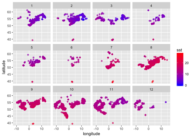
You can now plot sole occurrences by lon and lat, colour coded by temperature, faceted by month (1 = Jan to 12 = Dec) - this first requires defining a month variable:

sole_sst$month <- month(sole_sst$date)

Then create the plot like this:

(sole_sst_plot <- (ggplot(sole_sst, aes(x = longitude, y = latitude)) +
                     geom_point(aes(colour = sst), alpha = 2/3) +
                     scale_colour_gradient(low = "blue", high = "red") +
                     facet_wrap(~ month))
)

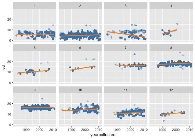
Alternatively you may want to look at trends over time in SST matched to sole occurrences, again faceted by month:

(sole_sst_trends <- ggplot(sole_sst, aes(x = yearcollected, y = sst)) +
  geom_point(colour = "steelblue", alpha = 1/3) +
  geom_smooth(method = "lm", colour = "darkorange") +
  facet_wrap(~ month)
)

🔗 Adding geography

All of the examples above have been global in scale, meaning that we have placed no spatial restrictions on the queries to OBIS - we have simply requested all occurrences that have been recorded anywhere on earth. However, we are frequently interested in sub-global analyses, either extracting data for an individual region of interest (such as a specific country’s EEZ), or summarising global data by region (e.g. records per regional sea). Here we show how OBIS queries can be refined using specific geometries, either supplied manually or as named regions obtained from the Marine Regions database. In these examples we return all records for a focal species within a region of interest, and also return a full species list for a focal region. In our original post we also showed how to combine geographic and environmental filters, for example returning all species occurring in regions of the North Atlantic that are <1000m deep.

Start by loading additional required packages:

library(rgdal)
library(mregions)
library(rgeos)
library(broom)

Get the UK EEZ shape file from marineregions:

uk_eez <- mr_shp("MarineRegions:eez",
	maxFeatures = NULL, filter = "United Kingdom Exclusive Economic Zone")

For convenience, simplify this and convert it to a data frame:

uk_eez_simple <- SpatialPolygonsDataFrame(gSimplify(
	uk_eez, tol = 0.01, topologyPreserve = TRUE), data = uk_eez@data)
uk_eez_df <- tidy(uk_eez_simple)

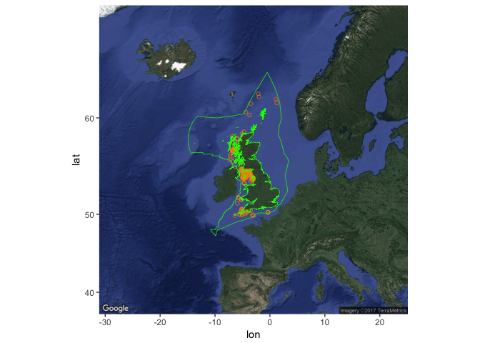
Get occurrences for a species (here, basking shark) within the UK EEZ:

basking_shark <- occurrence(
	scientificname = "Cetorhinus maximus", geometry = mr_as_wkt(uk_eez_simple))

Create the occurrence plot, then add the EEZ:

basking_map <- obis_map(basking_shark, map_type = "satellite", map_zoom = 4, plotit = F)
basking_map +
  geom_polygon(data = uk_eez_df, aes(x = long, y = lat, group = group),
               colour = "green", fill = NA, size = 0.25)

To get a list of species for a given region, use checklist, and specify your geometry (here an arbitrary 5 x 5 degree square in the NE Atlantic):

my_taxa <- tbl_df(checklist(
	geometry = "POLYGON ((-20 50, -20 55, -15 55, -15 50, -20 50))"))

Then filter this to taxa with species rank:

my_species <- filter(my_taxa, rank_name == "Species")

The result is a tibble of the 930 species found in this grid square, plus their full taxonomy and some additional summary information, including the number of records in OBIS (records):

my_species

## # A tibble: 930 × 18
##        id valid_id parent_id rank_name                   tname
##     <int>    <int>     <int>     <chr>                   <chr>
## 1  395754   395754    695236   Species     Acanthephyra eximia
## 2  395764   395764    695236   Species   Acanthephyra pelagica
## 3  395973   395973    395971   Species Acanthoica quattrospina
## 4  396173   396173    767483   Species Acanthoscina acanthodes
## 5  398225   398225    767500   Species      Adagnesia charcoti
## 6  398227   398227    767500   Species        Adagnesia rimosa
## 7  398647   398647    398644   Species        Aetideus armatus
## 8  400887   400887    400884   Species          Amperima rosea
## 9  401559   401559    738082   Species   Amphissa acutecostata
## 10 402079   402079    768595   Species      Amuletta abyssorum
## # ... with 920 more rows, and 13 more variables: tauthor <chr>,
## #   worms_id <int>, records <int>, datasets <int>, phylum <chr>,
## #   order <chr>, family <chr>, genus <chr>, species <chr>, class <chr>,
## #   redlist <lgl>, status <chr>, hab <lgl>

🔗 Next steps

The above describes some of the kinds of procedures that we use regularly in our group. Next steps could include further enrichment of occurrence data. For instance, there is a major initiative within WoRMS to link biological trait data to the existing taxonomy (see https://www.marinespecies.org/traits/) and we are thinking about how to filter OBIS queries by particular kinds of traits, or mapping the distribution of traits. We are also investigating how to mine the temporal dimension of OBIS data to derive robust estimates of trends in marine biodiversity. Keep an eye out for these developments on the OBIS news site, and please do get in touch with requests or suggestions for improvements!