Thursday, May 10, 2018 From rOpenSci (https://ropensci.org/blog/2018/05/10/onboarding-social-weather/). Except where otherwise noted, content on this site is licensed under the CC-BY license.
This blog post is the third of a 3-post series about a data-driven overview of rOpenSci onboarding. Read the intro to the series, the first post about data collection, the second post about quantifying work done by authors, reviewers and editors.
Our onboarding process ensures that packages contributed by the community undergo a transparent, constructive, non adversarial and open review process. Before even submitting my first R package to rOpenSci onboarding system in December 2015, I spent a fair amount of time reading through previous issue threads in order to assess whether onboarding was a friendly place for me: a newbie, very motivated to learn more but a newbie nonetheless. I soon got the feeling that yes, onboarding would help me make my package better without ever making me feel inadequate.
More recently, I read Anne Gentle’s essay in Open Advice where she mentions the concept of the social weather of an online community. By listening before I even posted, I was simply trying to get a good idea of the social weather of onboarding – as a side-note, how wonderful is it that onboarding’s being open makes it possible to listen?!
In the meantime, I’ve now only submitted and reviewed a few packages but also become an associate editor. In general, when one of us editors talks about onboarding, we like to use examples illustrating the system in a good light: often excerpts from review processes, or quotes of tweets by authors or reviewers. Would there be a more quantitative way for us to support our promotion efforts? In this blog post, I shall explore how a tidytext analysis of review processes (via their GitHub threads) might help us characterize the social weather of onboarding.
🔗 Preparing the data
🔗 A note about text mining
In this blog post, I’ll leverage the tidytext package, with the help
of its accompanying book “Tidy text
mining”. The authors, Julia Silge and
David Robinson, actually met and started working on this project, at
rOpenSci unconf in 2016!
🔗 The “tidy text” of the analysis
I’ve described in the first post of this series how I got all onboarding issue threads. Now, I’ll explain how I cleaned their text. Why does it need to be cleaned? Well, this text contains elements that I wished to remove: code chunks, as well as parts from our submission and review templates.
Edit: Find a cleaner approach to Markdown text extraction.
My biggest worry was the removal of templates from issues. I was already picturing my spending hours writing regular expressions to remove these lines… and then I realized that the word “lines” was the key! I could go split all issue comments into lines, which is called tokenization in proper text mining vocabulary, and then remove duplicates! This way, I didn’t even have to worry about the templates having changed a bit over time, since each version was used at least twice. A tricky part that remained was the removal of code chunks since I only wanted to keep human conversation. In theory, it was easy: code chunks are lines located between two lines containing “```”… I’m still not sure I solved this in the easiest possible way.
library("magrittr")
threads <- readr::read_csv("data/clean_data.csv")
# to remove code lines between ```
range <- function(x1, x2){
  x1:x2
}

# I need the indices of lines between ```
split_in_indices <- function(x){
  lengthx <- length(x)
  if(length(x) == 0){
    return(0)
  }else{
    if(lengthx > 2){

      limits1 <- x[seq(from = 1, to = (lengthx - 1), by = 2)]
      limits2 <- x[seq(from = 2, to = lengthx, by = 2)]
      purrr::map2(limits1, limits2, range) %>%
        unlist() %>%
        c()
    }else{
      x[1]:x[2]
    }
  }
}

# tokenize by line
threads <- tidytext::unnest_tokens(threads, line, body, token = "lines")

# remove white space
threads <- dplyr::mutate(threads, line = trimws(line))

# remove citations lines
threads <- dplyr::filter(threads, !stringr::str_detect(line, "^\\>"))

# remove the line from the template that has ``` that used to bother me
threads <- dplyr::filter(threads, !stringr::str_detect(line, "bounded by ```"))

# correct one line
threads <- dplyr::mutate(threads, line = stringr::str_replace_all(line, "`` `", "```"))

# group by comment
threads <- dplyr::group_by(threads, title, created_at, user, issue)

# get indices
threads <- dplyr::mutate(threads, index = 1:n())

# get lines limiting chunks
threads <- dplyr::mutate(threads, chunk_limit = stringr::str_detect(line, "```")&stringr::str_count(line, "`") %in% c(3, 4))

# special treatment
threads <- dplyr::mutate(threads,
                     chunk_limit = ifelse(user == "MarkEdmondson1234" & issue == 127 & index == 33,
                                          FALSE, chunk_limit))
threads <- dplyr::mutate(threads, which_limit = list(split_in_indices(which(chunk_limit))))

# weird code probably to get indices of code lines
threads <- dplyr::mutate(threads, code = index %in% which_limit[[1]])
threads <- dplyr::ungroup(threads)
Let’s look at what this does in practice, with comments from
gutenbergr
submission as
example. I chose this submission because the package author, David
Robinson, is one of the two tidytext creators, and because I was the
reviewer, so it’s all very meta, isn’t it?
In the excerpt below, we see the most important variable, the binary
code indicating whether the line is a code line. This excerpt also
shows variables created to help compute code: index is the index of
the line withing a comment, chunk_limit indicates whether the line is
a chunk limit, which_limit indicates which indices in the comment
indicate lines of code.
dplyr::filter(threads, package == "gutenbergr",
              user == "sckott",
              !stringr::str_detect(line, "ropensci..footer")) %>%
  dplyr::mutate(created_at = as.character(created_at)) %>%
  dplyr::select(created_at, line, code, index, chunk_limit, which_limit) %>%
  knitr::kable()
| created_at | line | code | index | chunk_limit | which_limit |
|---|---|---|---|---|---|
| 2016-05-02 17:04:56 | thanks for your submission @dgrtwo - seeking reviewers now | FALSE | 1 | FALSE | 0 |
| 2016-05-04 06:09:19 | reviewers: @masalmon | FALSE | 1 | FALSE | 0 |
| 2016-05-04 06:09:19 | due date: 2016-05-24 | FALSE | 2 | FALSE | 0 |
| 2016-05-12 16:16:38 | having a quick look over this now… | FALSE | 1 | FALSE | 0 |
| 2016-05-12 16:45:59 | @dgrtwo looks great. just a minor thing: | FALSE | 1 | FALSE | 3:7 |
| 2016-05-12 16:45:59 | gutenberg_get_mirror() throws a warning due to xml2, at this line https://github.com/ropensci/gutenbergr/blob/master/R/gutenberg_download.R#l213 | FALSE | 2 | FALSE | 3:7 |
| 2016-05-12 16:45:59 | ``` r | TRUE | 3 | TRUE | 3:7 |
| 2016-05-12 16:45:59 | warning message: | TRUE | 4 | FALSE | 3:7 |
| 2016-05-12 16:45:59 | in node_find_one(xnod**e, xdoc, xpath = xpath, nsmap = ns) : | TRUE | 5 | FALSE | 3:7 |
| 2016-05-12 16:45:59 | 101 matches for .//a: using first | TRUE | 6 | FALSE | 3:7 |
| 2016-05-12 16:45:59 | ``` | TRUE | 7 | TRUE | 3:7 |
| 2016-05-12 16:45:59 | wonder if it’s worth a suppresswarnings() there? | FALSE | 8 | FALSE | 3:7 |
| 2016-05-12 20:42:53 | great! | FALSE | 1 | FALSE | 3:5 |
| 2016-05-12 20:42:53 | - add the footer to your readme: | FALSE | 2 | FALSE | 3:5 |
| 2016-05-12 20:42:53 | ``` | TRUE | 3 | TRUE | 3:5 |
| 2016-05-12 20:42:53 | ``` | TRUE | 5 | TRUE | 3:5 |
| 2016-05-12 20:42:53 | - could you add url and bugreports entries to description, so people know where to get sources and report bugs/issues | FALSE | 6 | FALSE | 3:5 |
| 2016-05-12 20:42:53 | - update installation of dev versions to ropenscilabs/gutenbergr and any urls for the github repo to ropenscilabs instead of dgrtwo | FALSE | 7 | FALSE | 3:5 |
| 2016-05-12 20:42:53 | - go to the repo settings –> transfer ownership and transfer to ropenscilabs - note that all our newer pkgs go to ropenscilabs first, then when more mature we’ll move to ropensci | FALSE | 8 | FALSE | 3:5 |
| 2016-05-13 01:22:22 | nice, builds on at travis https://travis-ci.org/ropenscilabs/gutenbergr/ - you can keep appveyor builds under your acct, or i can start on mine, let me know | FALSE | 1 | FALSE | 0 |
| 2016-05-13 16:06:31 | updated badge link, started an appveyor account with ropenscilabs as account name - sent pr - though the build is failing, something about getting the current gutenberg url https://ci.appveyor.com/project/sckott/gutenbergr/build/1.0.1#l650 | FALSE | 1 | FALSE | 0 |
So as you see now getting rid of chunks is straightforward: the lines
with code == TRUE have to be deleted.
# remove them and get rid of now useless columns
threads <- dplyr::filter(threads, !code)
threads <- dplyr::select(threads, - code, - which_limit, - index, - chunk_limit)
Now on to removing template parts… I noticed that removing duplicates
was a bit too drastic because sometimes duplicates were poorly formatted
citations, e.g. an author answering a reviewer’s question by
copy-pasting it without Markdown
blockquotes,
in which case we definitely want to keep the first occurrence. Besides,
duplicates were sometimes very short sentences such as “great!” that are
not templates, that we therefore should keep. Therefore, for each line,
I counted how many times it occurred overall (no_total_occ), and in
how many issues it occurred (no_issues).
Let’s look at Joseph Stachelek’s review of
rrricanes
for instance.
dplyr::filter(threads, user == "jsta", is_review) %>%
  dplyr::select(line) %>%
  head() %>%
  knitr::kable()
| line |
|---|
| ## package review |
| - [x] as the reviewer i confirm that there are no conflicts of interest for me to review this work (if you are unsure whether you are in conflict, please speak to your editor before starting your review). |
| #### documentation |
| the package includes all the following forms of documentation: |
| - [x] a statement of need clearly stating problems the software is designed to solve and its target audience in readme |
| - [x] installation instructions: for the development version of package and any non-standard dependencies in readme |
Now if we clean up a bit…
threads <- dplyr::group_by(threads, line)
threads <- dplyr::mutate(threads, no_total_occ = n(),
                     no_issues = length(unique(issue)),
                     size = stringr::str_length(line))
threads <- dplyr::ungroup(threads)
threads <- dplyr::group_by(threads, issue, line)
threads <- dplyr::arrange(threads, created_at)
threads <- dplyr::filter(threads, no_total_occ <= 2,
                     # for repetitions in total keep the short ones
                     # bc they are stuff like "thanks" so not template
                     # yes 10 is arbitrary
                     no_issues <= 1 | size < 10)
# when there's a duplicate in one issue
# it's probably citation
# so keep the first occurrence
get_first <- function(x){
  x[1]
}
threads <- dplyr::group_by(threads, issue, line)
threads <- dplyr::summarise_all(threads, get_first)
threads <- dplyr::select(threads, - no_total_occ, - size, - no_issues)

threads <- dplyr::mutate(threads, # let code words now be real words
                     line = stringr::str_replace_all(line, "`", ""),
                     # only keep text from links, not the links themselves
                     line = stringr::str_replace_all(line, "\\]\\(.*\\)", ""),
                     line = stringr::str_replace_all(line, "\\[", ""),
                     line = stringr::str_replace_all(line, "blob\\/master", ""),
                     # ’
                     line = stringr::str_replace_all(line, "’", ""),
                     # remove some other links
                     line = stringr::str_replace_all(line, "https\\:\\/\\/github\\.com\\/", ""))

threads <- dplyr::filter(threads, !stringr::str_detect(line, "estimated hours spent reviewing"))
threads <- dplyr::filter(threads, !stringr::str_detect(line, "notifications@github\\.com"))
threads <- dplyr::filter(threads, !stringr::str_detect(line, "reply to this email directly, view it on"))
threads <- dplyr::ungroup(threads)
Here is what we get from the same review.
dplyr::filter(threads, user == "jsta", is_review)  %>%
  dplyr::select(line) %>%
  head() %>%
  knitr::kable()
| line |
|---|
| * also, you might consider using the skip_on_cran function for lines that call an external download as recommended by the ropensci packaging guide. |
| * i am having timeout issues with building the getting_started vignette. i wonder if there is a particular year with very few hurricanes that would solve the timeout problem. |
| * i cannot build the data.world vignette. probably because i don’t have an api key set up. you may want to consider setting the code chunks to eval=false. |
| * i really like the tidy_ functions. i wonder if it would make it easier on the end-user to have the get_ functions return tidy results by default with an optional argument to return “messy” results. |
| * missing a maintainer field in the description |
| * there are no examples for knots_to_mph, mb_to_in, status_abbr_to_str, get_discus, get_fstadv, tidy_fstadv, tidy_wr, tidy_fcst. maybe some can be changed to non-exported? |
So now, we mostly got the interesting human and original language.
This got me “tidy enough” text. Let’s not mention this package author who found a way to poorly format their submission right under a guideline explaining how to copy the DESCRIPTION… Yep, that’s younger me. Oh well.
🔗 Computing sentiment
Another data preparation part was to compute the sentiment score of each
line via the sentimentr
package by Tyler Rinker, which computes a score for sentences, not for
single words.
sentiment <- all %>%
  dplyr::group_by(line, created_at, user, role, issue) %>%
  dplyr::mutate(sentiment = median(sentimentr::sentiment(line)$sentiment)) %>%
  dplyr::ungroup() %>%
  dplyr::select(line, created_at, user, role, issue, sentiment)
This dataset of sentiment will be used later in the post.
🔗 Tidy text analysis of onboarding social weather
🔗 What do reviews talk about?
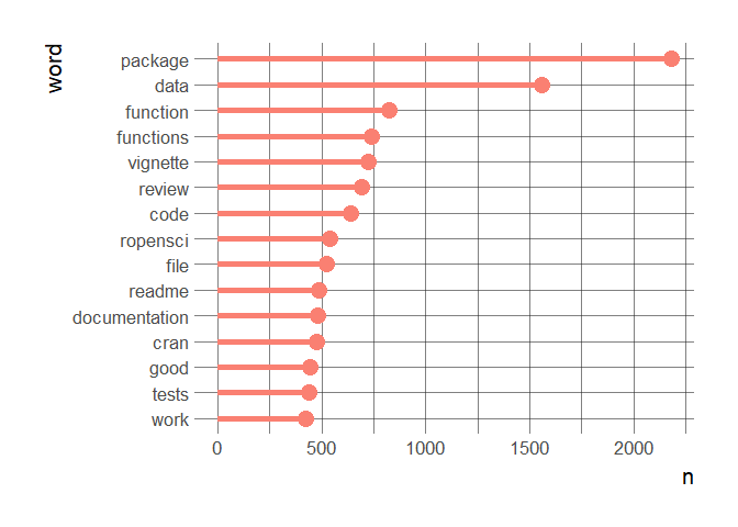
To find out what reviews deal with as if I didn’t know about our guidelines, I’ll compute the frequency of words and bigrams, and the pairwise correlation of words within issue comments.
My using lollipops below was inspired by this fascinating blog post of Tony ElHabr’s about his Google search history.
library("ggplot2")
library("ggalt")
library("hrbrthemes")

stopwords <- rcorpora::corpora("words/stopwords/en")$stopWords

word_counts <- threads %>%
  tidytext::unnest_tokens(word, line) %>%
  dplyr::filter(!word %in% stopwords) %>%
  dplyr::count(word, sort = TRUE) %>%
  dplyr::mutate(word = reorder(word, n))

ggplot(word_counts[1:15,]) +
  geom_lollipop(aes(word, n),
                size = 2, col = "salmon") +
  hrbrthemes::theme_ipsum(base_size = 16,
                          axis_title_size = 16) +
  coord_flip()
bigrams_counts <- threads %>%
  tidytext::unnest_tokens(bigram, line, token = "ngrams", n = 2) %>%
  tidyr::separate(bigram, c("word1", "word2"), sep = " ",
                  remove = FALSE) %>%
  dplyr::filter(!word1 %in% stopwords) %>%
  dplyr::filter(!word2 %in% stopwords) %>%
  dplyr::count(bigram, sort = TRUE) %>%
  dplyr::mutate(bigram = reorder(bigram, n))

ggplot(bigrams_counts[2:15,]) +
  geom_lollipop(aes(bigram, n),
                size = 2, col = "salmon") +
  hrbrthemes::theme_ipsum(base_size = 16,
                          axis_title_size = 16) +
  coord_flip()
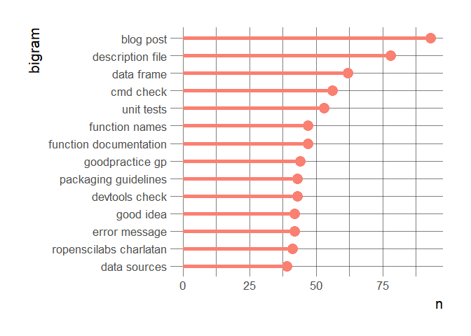
I’m not showing the first bigram that basically shows I’ve an encoding issue to solve with a variation of “´”. In any case, both figures show what we care about, like our guidelines that are mentioned often, and documentation. I think words absent from the figures such as performance or speed also highlight what we care less about, following Jeff Leek’s philosophy.
Now, let’s move on to a bit more complex visualization of pairwise correlations between words within lines. First, let’s prepare the table of words in lines. Compared with the book tutorial, we add a condition for eliminating words mentioned in only one submission, often function names.
users <- unique(threads$user)
onboarding_line_words <- threads %>%
  dplyr::group_by(user, issue, created_at, package, line) %>%
  dplyr::mutate(line_id = paste(package, user, created_at, line)) %>%
  dplyr::ungroup() %>%
  tidytext::unnest_tokens(word, line) %>%
  dplyr::filter( word != package, !word %in% users,
                 is.na(as.numeric(word)),
                 word != "ldecicco",
                 word != "usgs") %>%
  dplyr::group_by(word) %>%
  dplyr::filter(length(unique(issue)) > 1) %>%
  dplyr::select(line_id, word)

onboarding_line_words %>%
  head() %>%
  knitr::kable()
| line_id | word |
|---|---|
| rrlite karthik 2015-04-12 20:56:04 - ] add a ropensci footer. | add |
| rrlite karthik 2015-04-12 20:56:04 - ] add a ropensci footer. | a |
| rrlite karthik 2015-04-12 20:56:04 - ] add a ropensci footer. | ropensci |
| rrlite karthik 2015-04-12 20:56:04 - ] add a ropensci footer. | footer |
| rrlite karthik 2015-04-12 20:56:04 - ] add an appropriate entry into ropensci.org/packages/index.html | add |
| rrlite karthik 2015-04-12 20:56:04 - ] add an appropriate entry into ropensci.org/packages/index.html | an |
Then, we can compute the correlation.
word_cors <- onboarding_line_words %>%
  dplyr::group_by(word) %>%
  dplyr::filter(!word %in% stopwords) %>%
  dplyr::filter(n() >= 20) %>%
  widyr::pairwise_cor(word, line_id, sort = TRUE)
For instance, what often goes in the same line as vignette?
dplyr::filter(word_cors, item1 == "vignette")
## # A tibble: 853 x 3
##    item1    item2     correlation
##    <chr>    <chr>           <dbl>
##  1 vignette readme         0.176
##  2 vignette vignettes      0.174
##  3 vignette chunk          0.145
##  4 vignette eval           0.120
##  5 vignette examples       0.108
##  6 vignette overview       0.0933
##  7 vignette building       0.0914
##  8 vignette link           0.0863
##  9 vignette maps           0.0840
## 10 vignette package        0.0831
## # ... with 843 more rows
Now let’s plot the network of these relationships between words, using
the igraph package by Gábor Csárdi and Támas
Nepusz and ggraph package by
Thomas Lin Pedersen.
library("igraph")
library("ggraph")

set.seed(2016)

word_cors %>%
  dplyr::filter(correlation > .35) %>%
  graph_from_data_frame() %>%
  ggraph(layout = "fr") +
  geom_edge_link(aes(edge_alpha = correlation), show.legend = FALSE) +
  geom_node_point(color = "lightblue", size = 5) +
  geom_node_text(aes(label = name), repel = TRUE) +
  theme_void()
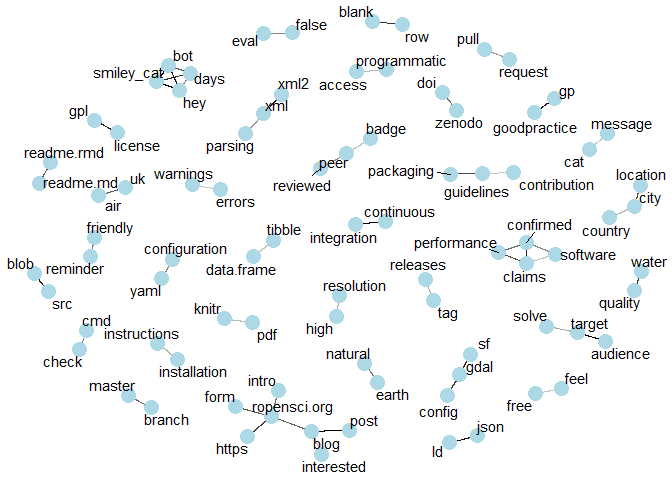
This figure gives a good sample of things discussed in reviews. Despite
our efforts filtering words specific to issues, some of them remain very
specific, such as country/city/location that are very frequent in
ropenaq review.
🔗 How positive is onboarding?
Using sentiment analysis, we can look at how positive comments are.
sentiments %>%
  dplyr::group_by(role) %>%
  skimr::skim(sentiment)
## Skim summary statistics
##  n obs: 11553
##  n variables: 6
##  group variables: role
##
## Variable type: numeric
##               role  variable missing complete    n  mean   sd   min p25
##             author sentiment       0     4823 4823 0.07  0.21 -1.2    0
##  community_manager sentiment       0       97   97 0.13  0.21 -0.41   0
##             editor sentiment       0     1521 1521 0.13  0.22 -1.63   0
##              other sentiment       0      344  344 0.073 0.2  -0.6    0
##           reviewer sentiment       0     4768 4768 0.073 0.21 -1      0
##  median  p75  max     hist
##   0     0.17 1.84 <U+2581><U+2581><U+2582><U+2587><U+2581><U+2581><U+2581><U+2581>
##   0.071 0.23 1    <U+2581><U+2581><U+2587><U+2585><U+2582><U+2581><U+2581><U+2581>
##   0.075 0.25 1.13 <U+2581><U+2581><U+2581><U+2581><U+2587><U+2586><U+2581><U+2581>
##   0     0.2  0.81 <U+2581><U+2581><U+2582><U+2587><U+2582><U+2582><U+2581><U+2581>
##   0     0.17 1.73 <U+2581><U+2581><U+2587><U+2585><U+2581><U+2581><U+2581><U+2581>
summary(sentiments$sentiment)
##     Min.  1st Qu.   Median     Mean  3rd Qu.     Max.
## -1.63200  0.00000  0.00000  0.07961  0.18353  1.84223
sentiments %>%
  dplyr::filter(!role %in% c("other", "community_manager")) %>%
  ggplot(aes(role, sentiment)) +
  geom_boxplot(fill = "salmon") +
  hrbrthemes::theme_ipsum(base_size = 16,
                          axis_title_size = 16,
                          strip_text_size = 16)
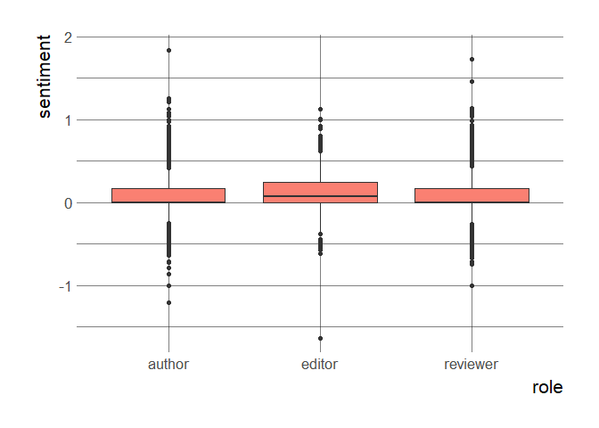
These boxplots seem to indicate that lines are generally positive (positive mean, zero 25th-quantile), although it’d be better to be able to compare them with text from traditional review processes of scientific manuscripts in order to get a better feeling for the meaning of these numbers.
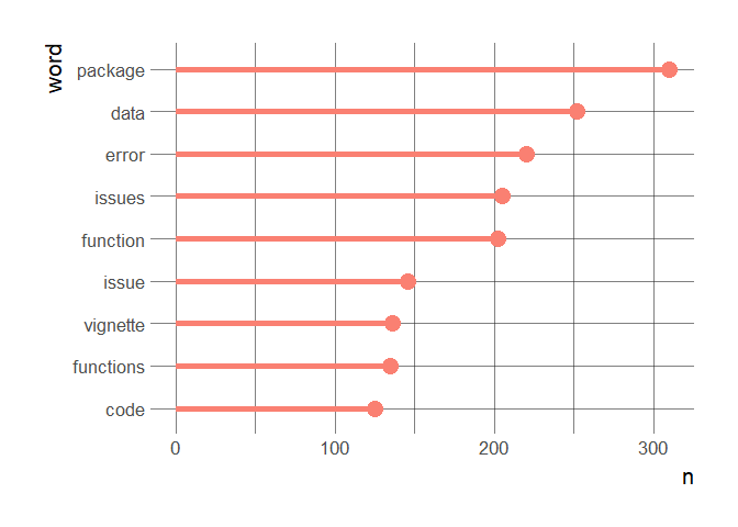
On these boxplots we also see that we do get lines with a negative sentiment value… about what? Here are the most common words in negative lines.
sentiments %>%
  dplyr::filter(sentiment < 0) %>%
  tidytext::unnest_tokens(word, line) %>%
  dplyr::filter(!word %in% stopwords) %>%
  dplyr::count(word, sort = TRUE) %>%
  dplyr::mutate(word = reorder(word, n)) %>%
  dplyr::filter(n > 100) %>%
ggplot() +
  geom_lollipop(aes(word, n),
                size = 2, col = "salmon") +
  hrbrthemes::theme_ipsum(base_size = 16,
                          axis_title_size = 16) +
  coord_flip()
And looking at a sample…
sentiments %>%
  dplyr::arrange(sentiment) %>%
  dplyr::select(line, sentiment) %>%
  head(n = 15) %>%
  knitr::kable()
| line | sentiment |
|---|---|
| @ultinomics no more things, although do make sure to add more examples - perhaps open an issue ropenscilabs/gtfsr/issues to remind yourself to do that, | -1.6320000 |
| not sure what you mean, but i’ll use different object names to avoid any confusion (ropenscilabs/mregions#24) | -1.2029767 |
| error in .local(.object, …) : | -1.0000000 |
| error: | -1.0000000 |
| #### miscellaneous | -1.0000000 |
| error: command failed (1) | -0.8660254 |
| - get_plate_size_from_number_of_columns: maybe throwing an error makes more sense than returning a string indicating an error | -0.7855844 |
| this code returns an error, which is good, but it would be useful to return a more clear error. filtering on a non-existant species results in a 0 “length” onekp object (ok), but then the download_* functions return a curl error due to a misspecified url. | -0.7437258 |
| 0 errors | 0 warnings | 0 notes | -0.7216878 |
| once i get to use this package more, i’m sure i’ll have more comments/issues but for the moment i just want to get this review done so it isn’t a blocker. | -0.7212489 |
| - i now realize i’ve pasted the spelling mistakes without thinking too much about us vs. uk english, sorry. | -0.7071068 |
| minor issues: | -0.7071068 |
| ## minor issues | -0.7071068 |
| replicates issue | -0.7071068 |
| visualization issue | -0.7071068 |
It seems that negative lines are mostly people discussing bugs and problems in code, and GitHub issues, and trying to solve them. The kind of negative lines we’re happy to see in our process, since once solved, they mean the software got more robust!
Last but not least, I mentioned our using particular cases as examples of how happy everyone seems to be in the process. To find such examples, we rely on memory, but what about picking heart-warming lines using their sentiment score?
sentiments %>%
  dplyr::arrange(- sentiment) %>%
  dplyr::select(line, sentiment) %>%
  head(n = 15) %>%
  knitr::kable()
| line | sentiment |
|---|---|
| absolutely - it’s really important to ensure it really has been solved! | 1.842234 |
| overall, really easy to use and really nicely done. | 1.733333 |
| this package is a great and lightweight addition to working with rdf and linked data in r. coming after my review of the codemetar package which introduced me to linked data, i found this a great learning experience into a topic i’ve become really interested in but am still quite novice in so i hope my feedback helps to appreciate that particular pov. | 1.463226 |
| i am very grateful for your approval and i very much look forward to collaborating with you and the ropensci community. | 1.256935 |
| thank you very much for the constructive thoughts. | 1.237437 |
| thanks for the approval, all in all a very helpful and educational process! | 1.217567 |
| - really good use of helper functions | 1.139013 |
| - i believe the utf note is handled correctly and this is just a snafu in goodpractice, but i will seek a reviewer with related expertise in ensuring that all unicode is handled properly. | 1.132201 |
| seem more unified and consistent. | 1.126978 |
| very much appreciated! | 1.125833 |
| - well organized, readable code | 1.100000 |
| - wow very extensive testing! well done, very thorough | 1.100000 |
| - i’m delighted that you find my work interesting and i’m very keen to help, contribute and collaborate in any capacity. | 1.084493 |
| thank you very much for your thorough and thoughtful review, @batpigandme ! this is great feedback, and i think that visdat will be much improved because of these reviews. | 1.083653 |
| great, thank you very much for accepting this package. i am very grateful about the reviews, which were very helpful to improve this package! | 1.074281 |
As you can imagine, these sentences make the whole team very happy! And we hope they’ll encourage you to contribute to rOpenSci onboarding.
🔗 Outlook
This first try at text analysis of onboarding issue threads is quite promising: we were able to retrieve text and to use natural language processing to extract most common words and bigrams, and sentiment. This allowed us to describe the social weather of onboarding: we could see that this system is about software, and that negative sentiment was often due to bugs being discussed and solved; and we could extract the most positive lines where volunteers praised the review system or the piece of software under review.
One could expand this analysis with a study of emoji use, in the text
using an emoji dictionary as in this blog
post and around the
text (so-called emoji reactions, present in the API and used in e.g
ghrecipes::get_issues_thumbs).
Another aspect of social weather is maybe the timeliness that’s expected
or implemented at the different parts of the process, but it’d be
covered by other data such as the labelling history of the issues, which
could get extracted from GitHub V4 API as well.
This is the final post of the “Our package review system in review” series. The first post presented data collection from GitHub, the second post aimed at quantifying the work represented by onboarding. The posts motivated us to keep using data to illustrate and assess the system. Brace yourself for more onboarding data analyses in the future!

