
Friday, May 18, 2018 From rOpenSci (https://ropensci.org/blog/2018/05/18/drake-hpc/). Except where otherwise noted, content on this site is licensed under the CC-BY license.
The drake R package is not only a reproducible research solution, but also a serious high-performance computing engine. The package website introduces drake, and this technical note draws from the guides on high-performance computing and timing in the drake manual.
🔗 You can help!
Some of these features are brand new, and others are newly refactored. The GitHub version has all the advertised functionality, but it needs more testing and development before I can submit it to CRAN in good conscience. New issues such as r-lib/processx#113 and HenrikBengtsson/future#226 seem to affect drake, and more may emerge. If you use drake for your own work, please consider supporting the project by field-testing the claims below and posting feedback here.
🔗 Let drake schedule your targets.
A typical workflow is a sequence of interdependent data transformations.
When you call make() on this project, drake takes care of "raw_data.xlsx", then raw_data, and then data in sequence. Once data completes, fit and hist can launch in parallel, and then "report.md" begins once everything else is done. It is drake’s responsibility to deduce this order of execution, hunt for ways to parallelize your work, and free you up to focus on the substance of your research.
🔗 Activate parallel processing.
Simply set the jobs argument to an integer greater than 1. The following make() recruits multiple processes on your local machine.
make(plan, jobs = 2)
For parallel deployment to a computing cluster (SLURM, TORQUE, SGE, etc.) drake calls on packages future, batchtools, and future.batchtools. First, create a batchtools template file to declare your resource requirements and environment modules. There are built-in example files in drake, but you will likely need to tweak your own by hand.
drake_batchtools_tmpl_file("slurm") # Writes batchtools.slurm.tmpl.
Next, tell future.batchtools to talk to the cluster.
library(future.batchtools)
future::plan(batchtools_slurm, template = "batchtools.slurm.tmpl")
Finally, set make()’s parallelism argument equal to "future" or "future_lapply".
make(plan, parallelism = "future", jobs = 8)
🔗 Choose a scheduling algorithm.
The parallelism argument of make() controls not only where to deploy the workers, but also how to schedule them. The following table categorizes the 7 options.
| Deploy: local | Deploy: remote | |
|---|---|---|
| Schedule: persistent | “mclapply”, “parLapply” | “future_lapply” |
| Schedule: transient | “future”, “Makefile” | |
| Schedule: staged | “mclapply_staged”, “parLapply_staged” | |
🔗 Staged scheduling
drake’s first custom parallel algorithm was staged scheduling. It was easier to implement than the other two, but the workers run in lockstep. In other words, all the workers pick up their targets at the same time, and each worker has to finish its target before any worker can move on. The following animation illustrates the concept.
But despite weak parallel efficiency, staged scheduling remains useful because of its low overhead. Without the bottleneck of a formal master process, staged scheduling blasts through armies of tiny conditionally independent targets. Consider it if the bulk of your work is finely diced and perfectly parallel, maybe if your dependency graph is tall and thin.
library(dplyr)
library(drake)

N <- 500

gen_data <- function() {
  tibble(a = seq_len(N), b = 1, c = 2, d = 3)
}

plan_data <- drake_plan(
  data = gen_data()
)

plan_sub <-
  gen_data() %>%
  transmute(
    target = paste0("data", a),
    command = paste0("data[", a, ", ]")
  )

plan <- bind_rows(plan_data, plan_sub)
plan
## # A tibble: 501 x 2
##    target command
##
##  1 data   gen_data()
##  2 data1  data[1, ]
##  3 data2  data[2, ]
##  4 data3  data[3, ]
##  5 data4  data[4, ]
##  6 data5  data[5, ]
##  7 data6  data[6, ]
##  8 data7  data[7, ]
##  9 data8  data[8, ]
## 10 data9  data[9, ]
## # ... with 491 more rows

config <- drake_config(plan)
vis_drake_graph(config)
🔗 Persistent scheduling
Persistent scheduling is brand new to drake. Here, make(jobs = 2) deploys three processes: two workers and one master. Whenever a worker is idle, the master assigns it the next target whose dependencies are fully ready. The workers keep running until no more targets remain. See the animation below.
🔗 Transient scheduling
If the time limits of your cluster are too strict for persistent workers, consider transient scheduling, another new arrival. Here, make(jobs = 2) starts a brand new worker for each individual target. See the following video.
🔗 How many jobs should you choose?
The predict_runtime() function can help. Let’s revisit the mtcars example.
Let’s also
- Plan for non-staged scheduling,
- Assume each non-file target (black circle) takes 2 hours to build, and
- Rest assured that everything else is super quick.
When we declare the runtime assumptions with the known_times argument and cycle over a reasonable range of jobs, predict_runtime() paints a clear picture.
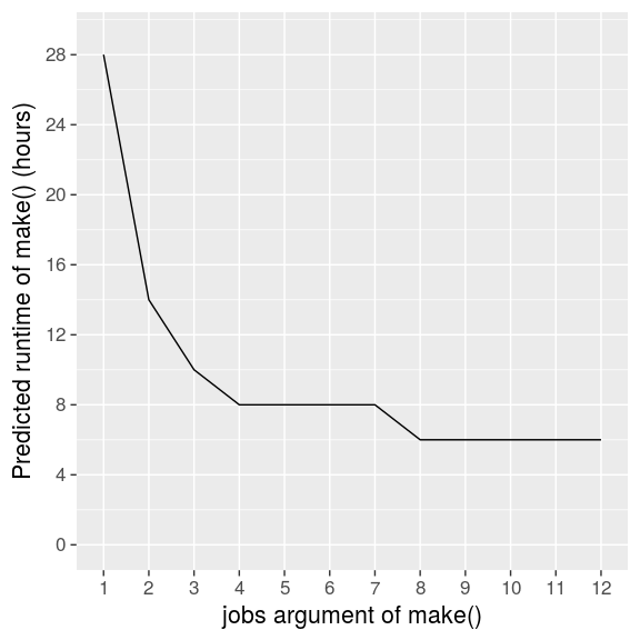
jobs = 4 is a solid choice. Any fewer would slow us down, and the next 2-hour speedup would take double the jobs and the hardware to back it up. Your choice of jobs for make() ultimately depends on the runtime you can tolerate and the computing resources at your disposal.
🔗 Thanks!
When I attended RStudio::conf(2018), drake relied almost exclusively on staged scheduling. Kirill Müller spent hours on site and hours afterwards helping me approach the problem and educating me on priority queues, message queues, and the knapsack problem. His generous help paved the way for drake’s latest enhancements.
🔗 Disclaimer
This post is a product of my own personal experiences and opinions and does not necessarily represent the official views of my employer. I created and embedded the Powtoon videos only as explicitly permitted in the Terms and Conditions of Use, and I make no copyright claim to any of the constituent graphics.
Filed under
Suggest an edit
Open a pull request
