Exploring European attitudes and behaviours using the European Social Survey

🔗 Introduction

I never thought that I’d be programming software in my career. I started using R a little over 2 years now and it’s been one of the most important decisions in my career. Secluded in a small academic office with no one to discuss/interact about my new hobby, I started searching the web for tutorials and packages. After getting to know how amazing and nurturing the R community is, it made me want to become a data scientist. So I set out to do it. Throughout the journey I repeatedly found myself using the European Social Survey (ESS from now on), a really neat dataset that collects information on attitudes, beliefs and behaviour patterns of diverse populations in more than thirty European nations since 2002.

After seeing a niche in the R package community, I created the package essurvey (previously ess in CRAN) to access this data easily from R. The package was accepted in CRAN in September 2017 and was well received among social scientists.

The 4th of March of 2018 I submitted the package to rOpensci, intimidated but very excited about the peer review process. To my surprise, the process was enriching, respectful and transparent, unlike my previous experience in academic research.

🔗 First steps

Using the essurvey package is fairly easy. There are are two main families of functions: import_* and show_*. They complement each other and allow the user to almost never have to go to the ESS website. The only scenario where you need to enter is to register your new account. If you haven’t registered, create an account at https://www.europeansocialsurvey.org/user/new and validate through your email inbox.

You can install the development version with

# install.packages("devtools")
devtools::install_github("ropensci/essurvey")

or the stable version from CRAN with

install.packages("essurvey")

Let’s load the CRAN version and load it together with the tidyverse set of packages to do some data manipulation.

library(essurvey)
library(tidyverse)

Given that some essurvey functions require your email address, this vignette will use a fake email but everything should work accordingly if you registered with the ESS. We can set our email as an environment variable with set_email

set_email("[email protected]")

Before we continue, let’s briefly explain some terminology of the ESS data. Surveys are carried out every 2 years and each survey is called rounds or waves. For example, round one was the first round ever implemented, which dates back to 2002. The second round followed up in 2004 and it’s usually referred to as second round or second wave. There are currently eight rounds freely available.

The ESS has over a thousand questions that include interesting topics such as attitudes towards national governments, democracy, immigration, nationalism, public policy as well demographic and subjective health data on the participants of the survey. Most of these questions use likert-type scales which means that the possible answers to any given question range either from 0 through 5 or 0 through 10. For example, an average question would be something like: how satisfied are you with democracy in your country? and the possible answers range from 0 to 10 where 0 means very unsatisfied and 10 very satisfied.

🔗 Exploring government satisfacion in Spain

Let’s suppose you don’t know which countries or rounds (waves) are available for the ESS. Then the show_* family of functions is your friend.

To find out which countries have participated you can use show_countries()

show_countries()

##  [1] "Albania"            "Austria"            "Belgium"           
##  [4] "Bulgaria"           "Croatia"            "Cyprus"            
##  [7] "Czech Republic"     "Denmark"            "Estonia"           
## [10] "Finland"            "France"             "Germany"           
## [13] "Greece"             "Hungary"            "Iceland"           
## [16] "Ireland"            "Israel"             "Italy"             
## [19] "Kosovo"             "Latvia"             "Lithuania"         
## [22] "Luxembourg"         "Netherlands"        "Norway"            
## [25] "Poland"             "Portugal"           "Romania"           
## [28] "Russian Federation" "Slovakia"           "Slovenia"          
## [31] "Spain"              "Sweden"             "Switzerland"       
## [34] "Turkey"             "Ukraine"            "United Kingdom"

This function actually looks up the countries in the ESS website. If new countries enter, this will automatically grab those countries as well. Let’s check out Spain. How many rounds has Spain participated in? We can use show_country_rounds()

sp_rnds <- show_country_rounds("Spain")
sp_rnds

## [1] 1 2 3 4 5 6 7

Note that country names are case sensitive. Use the exact name printed out by show_countries().

Using this information, we can download those specific rounds easily with import_country.

spain <-
  import_country(
    country = "Spain",
    rounds = 1:7
    )

Note: Since essurvey 1.0.0 all ess_* functions have been deprecated in favour of the import_* and download_* functions.

spain will now be a list of length(rounds) containing a data frame for each round. The import_* family is concerned with downloading the data and thus always returns a list containing data frames unless only one round is specified, in which it returns a tibble. Conversely, the show_* family grabs information from the ESS website and always returns vectors.

To download all rounds for a country automatically you can use import_all_cntrounds.

import_all_cntrounds("Spain")

ESS datasets flag missing values differently between questions. For example, questions with possible answers ranging from 0 through 5 have missing categories such as “Don’t know” and “Refusal” coded as 7 and 8 and 9. But for questions with possible answers ranging from 0 through 10 missing values are coded as 77, 88 and 99. recode_missings accepts a tibble as a main argument and automatically returns a new tibble with all missing values recoded as NA. You should check out ?recode_missings for more details and elaborated examples.

Note: I urge the reader not to recode these categories to missing without previously investigating the importance of these categories.

For example, let’s recode missing values in all Spanish waves, bind them into one single tibble and visualize how satisfied are Spaniards with their government. First, let’s extract a cleaner data.

semi_cleaned <-
  spain %>% 
  map(recode_missings) %>% 
  bind_rows() %>% 
  mutate(name = str_sub(name, end = 4)) %>% 
  select(name, stfgov)

semi_cleaned

## # A tibble: 13,543 x 2
##    name  stfgov
##    <chr>  <dbl>
##  1 ESS1      0.
##  2 ESS1      0.
##  3 ESS1      5.
##  4 ESS1      5.
##  5 ESS1      4.
##  6 ESS1      7.
##  7 ESS1      2.
##  8 ESS1      2.
##  9 ESS1      3.
## 10 ESS1      3.
## # ... with 13,533 more rows

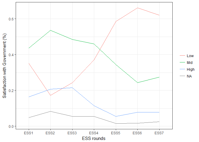
There we go. The scale of stfgov is between 0 and 10, where 0 means very unsatisfied with government and 10 very satisfied. Let’s collapse that into smaller categories, calculate the percentage of respondents within each category and visualize the change over time.

semi_cleaned %>% 
  mutate(stfgov = case_when(stfgov <= 3 ~ "Low",
                            between(stfgov, 4, 6) ~ "Mid",
                            stfgov >= 7 ~ "High"),
         stfgov = factor(stfgov, levels = c("Low", "Mid", "High"))) %>%
  count(name, stfgov) %>% 
  group_by(name) %>% 
  mutate(perc = n / sum(n)) %>% 
  ggplot(aes(name, perc, group = stfgov, colour = stfgov)) +
  geom_line() +
  theme_bw() +
  labs(x = "ESS rounds", y = "Satisfaction with Government (%)") +
  scale_colour_discrete(name = NULL)

Looks like Spaniards are increasingly unhappy with their government!

🔗 Exploring data by waves

Similarly to import_country, we can use other functions to download rounds containing all countries. To see which rounds are currently available, use show_rounds.

show_rounds()

## [1] 1 2 3 4 5 6 7 8

Similar to show_countries, show_rounds interactively looks up rounds in the ESS website, so any future rounds will automatically be included.

To download selected rounds, you can use import_rounds.

selected_rounds <- import_rounds(1:7)

Alternatively, use import_all_rounds to download all available rounds.

all_rounds <- import_all_rounds()

To build on the previous example, we can compare two different countries on their satisfaction with governments. Let’s map through each round, select our columns of interest, filter for Spain and France, and bind those data frames into one single tidy tibble.

semi_cleaned <-
  selected_rounds %>% 
  map(~ select(.x, name, cntry, stfgov)) %>% 
  map(~ filter(.x, cntry %in% c("ES","FR"))) %>% 
  bind_rows() %>% 
  mutate(name = str_sub(name, end = 4)) %>% 
  recode_missings()

semi_cleaned

## # A tibble: 26,524 x 3
##    name  cntry stfgov
##    <chr> <chr>  <dbl>
##  1 ESS1  ES        0.
##  2 ESS1  ES        0.
##  3 ESS1  ES        5.
##  4 ESS1  ES        5.
##  5 ESS1  ES        4.
##  6 ESS1  ES        7.
##  7 ESS1  ES        2.
##  8 ESS1  ES        2.
##  9 ESS1  ES        3.
## 10 ESS1  ES        3.
## # ... with 26,514 more rows

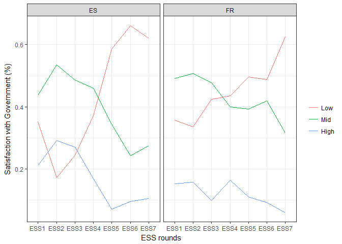
Now that we’ve got that down, let’s visualize the change over time by calculating the percentage of respondents in each category for every year/country combination and visualize the results.

semi_cleaned %>% 
  mutate(stfgov = case_when(stfgov <= 3 ~ "Low",
                            between(stfgov, 4, 6) ~ "Mid",
                            stfgov >= 7 ~ "High"),
         stfgov = factor(stfgov, levels = c("Low", "Mid", "High"))) %>%
  count(name, cntry, stfgov) %>% 
  group_by(name, cntry) %>% 
  mutate(perc = n / sum(n)) %>% 
  ggplot(aes(name, perc, group = stfgov, colour = stfgov)) +
  geom_line() +
  theme_bw() +
  labs(x = "ESS rounds", y = "Satisfaction with Government (%)") +
  scale_colour_discrete(name = NULL) +
  facet_wrap(~ cntry)

Spain and France follow very similar patterns although the changes are much steeper in Spain! A more elaborate analysis would perhaps be interested in finding out if this trend line is similar in other countries.

🔗 Downloading data for Stata, SPSS and SAS users

To finish off, all import_* functions have an equivalent download_* function that allows the user to save the datasets in a specified folder in 'stata', 'spss' or 'sas' formats.

For example, to save round two from Turkey in a folder called ./my_folder, we use:

download_country("Turkey", 2,
                 output_dir = "./myfolder/")

By default it saves the data as 'stata' files. Alternatively you can use 'spss' or 'sas'.

download_country("Turkey", 2,
                 output_dir = "./myfolder/",
                 format = 'sas')

This will save the data to ./myfolder/ESS_Turkey and inside that folder there will be the ESS2 folder that contains the data. The round equivalent is download_rounds

🔗 Analyzing ESS data

Be aware that for analyzing data from the ESS survey you should take into consideration the sampling and weights of each country/wave. The survey package provides very good support for this. A useful example comes from the work of Anthony Damico and Daniel Oberski here. This example calculated percentages manually and appropriate statistical inference should consider the above.

🔗 Acknowledgments

The package was improved greatly thanks to the reviews of Thomas Leeper and Nujcharee Haswell and editorial skills of Maëlle Salmon. I am indebted to their work. I would also like to thank Wiebke Weber at the Research and Expertise Centre for Survey Methodology for giving support and feedback in the development of the package.

The official package repository is at Github here. If you find any bugs or would like to request a feature, please file an issue there. The package is still very young and will most likely evolve in the near future. If you’re interested in contributing to the development essurvey, don’t hesitate to file a pull request which I’ll gladly review. One important feature that is still missing is being able to download the associated weight data for each country/wave. These files are called “SDDF” and can be found in the ESS website. For example, the SDDF files for some countries in round 6 can be found here.