phylogram: dendrograms for evolutionary analysis

Evolutionary biologists are increasingly using R for building, editing and visualizing phylogenetic trees. The reproducible code-based workflow and comprehensive array of tools available in packages such as ape, phangorn and phytools make R an ideal platform for phylogenetic analysis. Yet the many different tree formats are not well integrated, as pointed out in a recent post.

The standard data structure for phylogenies in R is the “phylo” object, a memory efficient, matrix-based tree representation. However, non-biologists have tended to use a tree structure called the “dendrogram”, which is a deeply nested list with node properties defined by various attributes stored at each level. While certainly not as memory efficient as the matrix-based format, dendrograms are versatile and intuitive to manipulate, and hence a large number of analytical and visualization functions exist for this object type. A good example is the dendextend package, which features an impressive range of options for editing dendrograms and plotting publication-quality trees.

To better integrate the phylo and dendrogram object types, and hence increase the options available for both camps, we developed the phylogram package, which is now a part of the rOpenSci project. This small package features a handful of functions for tree conversion, importing and exporting trees as parenthetic text, and manipulating dendrograms for phylogenetic applications. The phylogram package draws heavily on ape, but currently has no other non-standard dependencies.

\

🔗 Installation

To download phylogram from CRAN and load the package, run

install.packages("phylogram")
library(phylogram)

Alternatively, to download the latest development version from GitHub, first ensure that the devtools, kmer, and dendextend packages are installed, then run:

devtools::install_github("ropensci/phylogram", build_vignettes = TRUE) 
library(phylogram)

\

🔗 Tree import/export

A wide variety of tree formats can be parsed as phylo objects using either the well-optimized ape::read.tree function (for Newick strings), or the suite of specialized functions in the versatile treeio package. To convert a phylo object to a dendrogram, the phylogram package includes the function as.dendrogram, which retains node height attributes and can handle non-ultrametric trees.

For single-line parsing of dendrograms from Newick text, the read.dendrogram function wraps ape::read.tree and converts the resulting phylo class object to a dendrogram using as.dendrogram.

Similarly, the functions write.dendrogram and as.phylo are used to export dendrogram objects to parenthetic text and phylo objects, respectively.

\

🔗 Tree editing

The phylogram package includes some new functions for manipulating trees in dendrogram format. Leaf nodes and internal branching nodes can be removed using the function prune, which identifies and recursively deletes nodes based on pattern matching of “label” attributes. This is slower than ape::drop.tip, but offers the benefits of versatile string matching using regular expressions, and the ability to remove inner nodes (and by extension all subnodes) that feature matching “label” attributes. To aid visualization, the function ladder rearranges the tree, sorting nodes by the number of members (analogous to ape::ladderize).

For more controlled subsetting or when creating trees from scratch (e.g. from a standard nested list), the function remidpoint recursively corrects all “midpoint”, “members” and “leaf” attributes. Node heights can then be manipulated using either reposition, which scales the heights of all nodes in a tree by a given constant, or as.cladogram, which resets the “height” attributes of all terminal leaf nodes to zero and progressively resets the heights of the inner nodes in single incremental units.

As an example, a simple three-leaf dendrogram can be created from a nested list as follows:

x <- list(1, list(2, 3))
## set class, midpoint, members and leaf attributes for each node
x <- remidpoint(x)
## set height attributes for each node
x <- as.cladogram(x)

A nice feature of the dendrogram object type is that tree editing operations can be carried out recursively using fast inbuilt functions in the “apply” family such as dendrapply and lapply.

For example, to label each leaf node of the tree alphabetically we can create a simple labeling function and apply it to the tree nodes recursively using dendrapply.

set_label <- function(node){
  if(is.leaf(node)) attr(node, "label") <- LETTERS[node]
  return(node)
}
x <- dendrapply(x, set_label)
plot(x, horiz = TRUE)

🔗 Applications

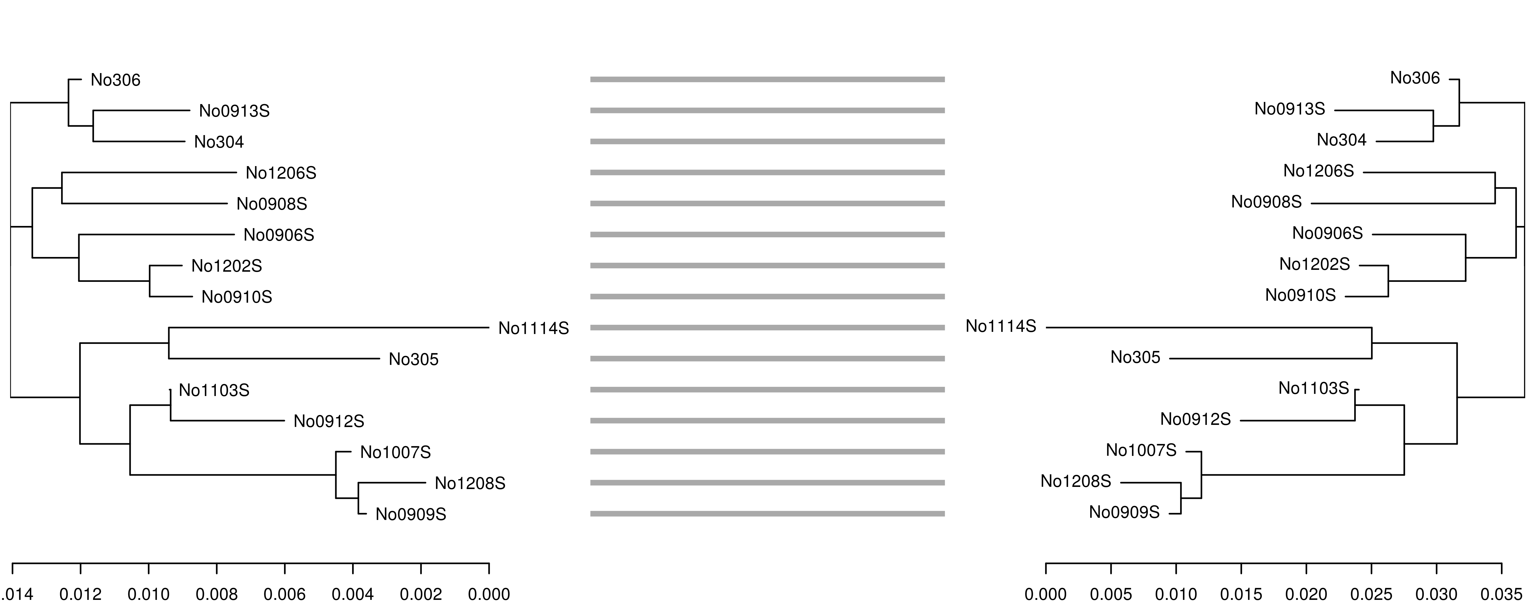
One application motivating bi-directional conversion between phylo and dendrogram objects involves creating publication-quality ’tanglegrams’ using the dendextend package. For example, to see how well the fast, alignment-free k-mer distance from the kmer package performs in comparison to the standard Kimura 1980 distance measure, we can create neighbor-joining trees using each method and plot them side by side to check for incongruent nodes.

## load woodmouse data and remove columns with ambiguities
data(woodmouse, package = "ape")
woodmouse <- woodmouse[, apply(woodmouse, 2, function(v) !any(v == 0xf0))]
## compute Kimura 1980 pairwise distance matrix
dist1 <- ape::dist.dna(woodmouse, model = "K80")
## deconstruct alignment (not strictly necessary)
woodmouse <- as.list(as.data.frame(unclass(t(woodmouse))))
## compute kmer distance matrix 
dist2 <- kmer::kdistance(woodmouse, k = 7) 
## build and ladderize neighbor-joining trees
phy1 <- ape::nj(dist1)
phy2 <- ape::nj(dist2)
phy1 <- ape::ladderize(phy1)
phy2 <- ape::ladderize(phy2)
## convert phylo objects to dendrograms
dnd1 <- as.dendrogram(phy1)
dnd2 <- as.dendrogram(phy2)
## plot the tanglegram
dndlist <- dendextend::dendlist(dnd1, dnd2)
dendextend::tanglegram(dndlist, fast = TRUE, margin_inner = 5)

\

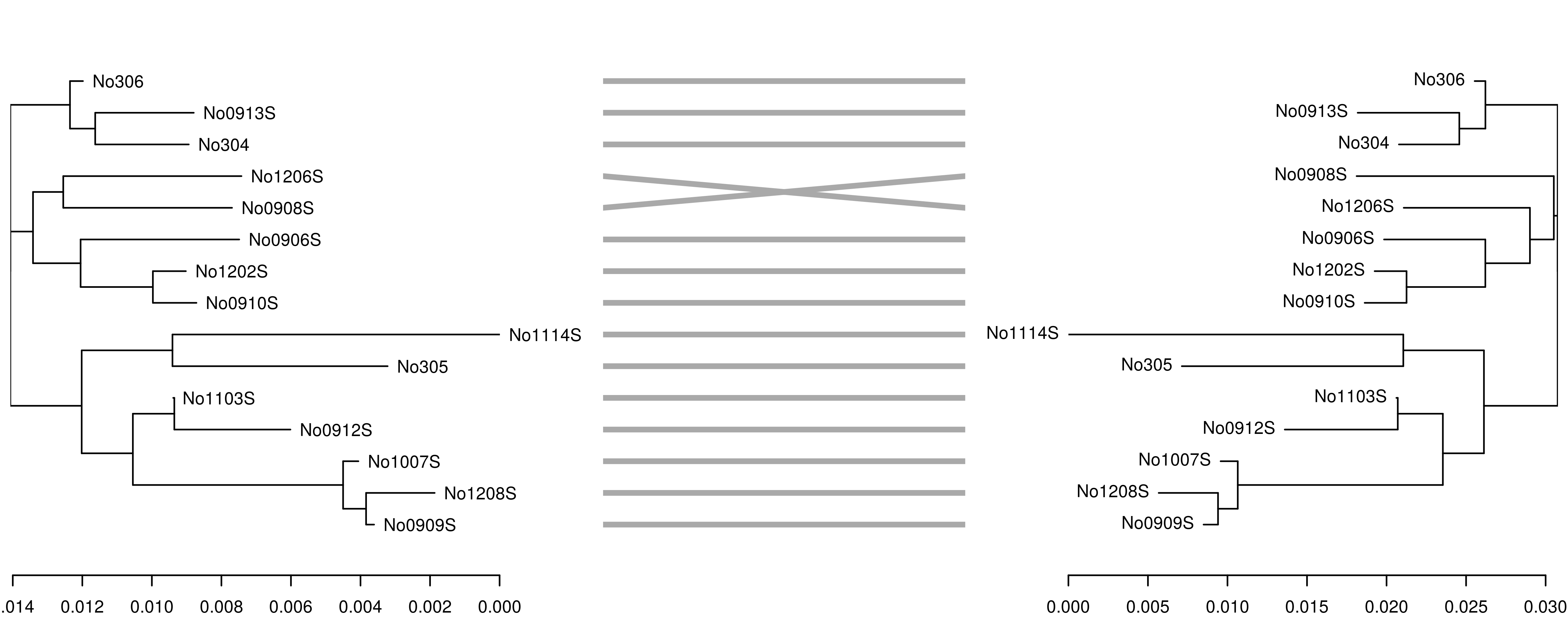
In this case, the trees are congruent and branch lengths are similar. However, if we reduce the k-mer size from 7 to 6, the accuracy of the tree reconstruction is affected, as shown by the incongruence between the original K80 tree (left) and the tree derived from the 6-mer distance matrix (right):

## compute kmer distance matrix 
dist3 <- kmer::kdistance(woodmouse, k = 6) 
phy3 <- ape::nj(dist3)
phy3 <- ape::ladderize(phy3)
dnd3 <- as.dendrogram(phy3)
dndlist <- dendextend::dendlist(dnd1, dnd3)
dendextend::tanglegram(dndlist, fast = TRUE, margin_inner = 5)

\

Hopefully users will find the package useful for a range of other applications. Bug reports and other suggestions are welcomed, and can be directed to the GitHub issues page or the phylogram google group. Thanks to Will Cornwell and Ben J. Ward for reviewing the code and suggesting improvements, and to Scott Chamberlain for handling the rOpenSci onboarding process.

The phylogram package is available for download from GitHub and CRAN, and a summary of the package is published in the Journal of Open Source Software.