
Wednesday, August 8, 2018 From rOpenSci (https://ropensci.org/blog/2018/08/08/phylotar/). Except where otherwise noted, content on this site is licensed under the CC-BY license.
In this technote I will outline what phylotaR was developed for, how to install it and how to run it with some simple examples.
🔗 What is phylotaR?
In any phylogenetic analysis it is important to identify sequences that share the same orthology – homologous sequences separated by speciation events. This is often performed by simply searching an online sequence repository using sequence labels. Relying solely on sequence labels, however, can miss sequences that have either not been labelled, have unanticipated names or have been mislabelled.
The phylotaR package, like its earlier inspiration PhyLoTa, identifies sequences of shared orthology not by naming matching but instead through the use of an alignment search tool, BLAST. As a result, a user of phylotaR is able to download more relevant sequence data for their phylogenetic analysis than they otherwise would.
From the taxon of interest the phylotaR pipeline traverses down the taxonomy and downloads entire subsets of sequences representing different nodes in the taxonomy. For taxa with too many sequences (e.g. Homo sapiens, Arabidopsis thaliana), a random subset is instead downloaded. For each of these subsets of downloaded sequences all-vs-all BLAST is then performed. The BLAST results of these subsets are parsed to identify all the independent, homologous clusters of sequences as determined using E-values and coverages. A secondary clustering step performs BLAST again to identify higher-level taxonomic clusters, above the level at which the all-vs-all BLAST searches were performed. This pipeline is automated and all a user needs to supply is a taxonomic group of interest from which the pipeline will begin its traverse. The pipeline is broken down into four stages: retrieve taxonomic information (’taxise’), download sequences, identify clusters and identify clusters among the clusters.
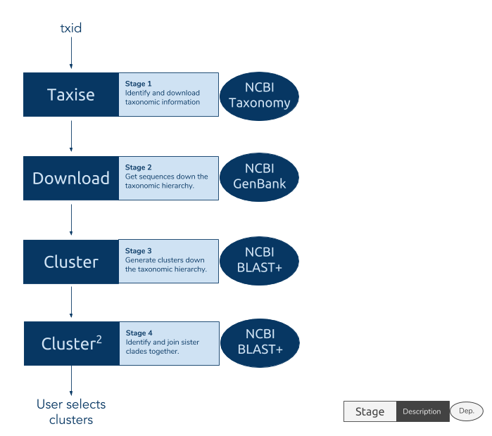 Figure 1. The stages of phylotaR pipeline: taxise, download, cluster and cluster^2. Note, ’taxise’ is the name of a stage and does not relate to the package
 taxize.
After a pipeline has completed, the package provides a series of tools for interacting with the results to identify potential ortholgous clusters suitable for phylogenetic analysis. These tools include methods for filtering based on sequence lengths, sequence annotations, taxonomy …etc. As well as for visualisations to, for example, check the relative abundance of sequences by taxon.
For more information on how the pipeline works, please see the open-access scientific article: phylotaR: An Automated Pipeline for Retrieving Orthologous DNA Sequences from GenBank in R
🔗 Installation
phylotaR is available from CRAN.
install.packages('phylotaR')
Alternatively, the latest development version can be downloaded from phylotaR’s GitHub page.
devtools::install_github(repo = 'ropensci/phylotaR', build_vignettes = TRUE)
🔗 BLAST+
In addition to the R package you will also need to have installed BLAST+ – a local copy of the well-known BLAST software on your machine. Unfortunately this can be a little complex as its installation depends on your operating system (Windows, Mac or Linux). Fortunately, NCBI provides detailed installation instructions for each flavour of operating system: NCBI installation instructions.
Once BLAST+ is installed you will need to record the location of the BLAST+ file system path where the exectuable programs are located. This should be something like C:\users\tao\desktop\blast-2.2.29+\bin\ on a Windows machine or /usr/local/ncbi/blast/bin/ on a Unix.
🔗 Quick guide
🔗 Taxonomic ID
After installation, a phylotaR pipeline can be launched with the setup() and run() functions. Before launching a run, a user must first look up the NCBI taxonomic ID for their chosen taxonomic group. To find the ID of your taxon, search NCBI taxonomy using the scientific name or an English common name. For example, upon searching for the primate genus ‘Aotus’ we should come across this page which states the taxonomic ID as 9504.
Because names are not unique phylotaR does not allow names to be used instead of taxonomic IDs. Aotus is a good example as there is also a plant genus of the same name. If we were to search NCBI with just the name then we would be downloading a mixture of primate and plant DNA. Such is the importance of IDs. (Alternatively, you could automate this step yourself using the taxize package.)
🔗 Running
With the package installed, BLAST+ available and ID to hand, we can run our pipeline.
# load phylotaR
library(phylotaR)
# create a folder to hold the cached data and results
dir.create('aotus')
# setup the folder and check that BLAST is available
setup(wd = wd, txid = 9504, ncbi_dr = '/usr/local/ncbi/blast/bin/')
# run the pipeline
run(wd = wd)
# ^^ running should take about 5 minutes to complete
For more details on running the pipeline, such as changing the parameters or understanding the results, see the vignette, vignette('phylotaR') or visit the website.
🔗 Timings
The time it takes for a pipeline to complete depends on the number of taxonomic groups a taxon contains and the number of sequences it represents. Below are some examples of the time taken for various taxonomic groups.
| Taxon | N. taxa | N. sequences | Time taken (mins.) |
|---|---|---|---|
| Anisoptera (“dragonflies”) | 1175 | 11432 | 72 |
| Acipenseridae (“sturgeons”) | 51 | 2407 | 13 |
| Tinamiformes (“tinamous”) | 25 | 251 | 2.7 |
| Aotus (“night/owl monkeys”) | 13 | 1499 | 3.9 |
| Bromeliaceae (“bromeliads”) | 1171 | 9833 | 66 |
| Cycadidae (“cycads”) | 353 | 8331 | 37 |
| Eutardigrada (“water bears”) | 261 | 960 | 14 |
| Kazachstania (a group of yeast) | 40 | 623 | 23 |
| Platyrrhini (“new world monkeys”) | 212 | 12731 | 60 |
🔗 Reviewing the results
After a pipeline has completed, the wd will contain all the results files. The information contained within these files can be read into the R environment using the read_phylota() function. It will generate a Phylota object that contains information on all the identified ‘clusters’ – i.e. groups of ortholgous sequences. A user can interact with the object to filter out unwanted sequences, clusters or taxonomic groups. The package comes with completed results for playing with. In the example below, we demonstrate how to generate a presence/absence matrix of all the genera in the top 10 clusters identifed for cycads, 1445963.
library(phylotaR)
data(cycads)
# drop all but first ten
cycads <- drop_clstrs(cycads, cycads@cids[1:10])
# get genus-level taxonomic names
genus_txids <- get_txids(cycads, txids = cycads@txids, rnk = 'genus')
genus_txids <- unique(genus_txids)
# dropping missing
genus_txids <- genus_txids[genus_txids !=  '']
genus_nms <- get_tx_slot(cycads, genus_txids, slt_nm = 'scnm')
# make alphabetical for plotting
genus_nms <- sort(genus_nms, decreasing = TRUE)
# generate geom_object
p <- plot_phylota_pa(phylota = cycads, cids = cycads@cids, txids = genus_txids,
                     txnms = genus_nms)
# plot
print(p)
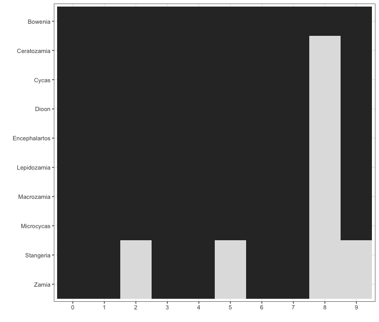 Figure 2. The presence (dark block) or absence (light block) for different cycad genera across the top ten clusters in the example dataset.
In this next example, we create a treemap showing the differences in the number of sequences and clusters identifed between genera in tinamous, 8802. (For the unintiated, tinamous are semi-flightless birds found in South America and members of the ratities – the same group comprising ostrichs and kiwis.)
library(phylotaR)
data(tinamous)
# Plot taxa, size by n. sq, fill by ncl
txids <- get_txids(tinamous, txids = tinamous@txids, rnk = 'genus')
txids <- txids[txids !=  '']
txids <- unique(txids)
txnms <- get_tx_slot(tinamous, txids, slt_nm = 'scnm')
p <- plot_phylota_treemap(phylota = tinamous, txids = txids, txnms = txnms,
                          area = 'nsq', fill = 'ncl')
print(p)
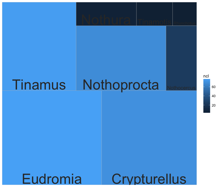 Figure 3. Relative number of sequences and clusters per tinamous genus. The larger the size of the box, the more sequences are represented for the genus. The lighter the blue colour, the more clusters are represented for the genus.
Through interacting with the Phylota object and using the various functions for manipulating it, a user can extract the specific ortholgous sequences of interest and write out the sequences in fasta format with the write_sqs() function.
# get sequences for a cluster and write out
data('aotus')
# take the first cluser ID
cid <- aotus@cids[[1]]
# extract its sequence IDs from Phylota object
sids <- aotus[[cid]]@sids
# design sequence names for definition line
sid_txids <- get_sq_slot(phylota = aotus, sid = sids, slt_nm = 'txid')
sid_spnms <- get_tx_slot(phylota = aotus, txid = sid_txids, slt_nm = 'scnm')
sq_nms <- paste0(sid_spnms, ' | ', sids)
# write out
write_sqs(phylota = aotus, outfile = file.path(tempdir(), 'test.fasta'),
          sq_nm = sq_nms, sid = sids)
For more information and examples on manipulating the Phylota object, see the phylotaR website.
🔗 Future
We have many ideas for improving phylotaR, such as making use of the BLAST API – instead of relying on users installing BLAST+ on their machine – and allowing users to introduce their own non-GenBank sequences. Please see the contributing page for a complete and current list of development options. Fork requests are welcome!
Alternatively, if you have any ideas of your own for new features than please open a new issue.
🔗 Acknowledgements
Big thanks to Zebulun Arendsee, Naupaka Zimmerman and Scott Chamberlain for reviewing/editing the package for ROpenSci.
🔗 Useful Links
- The phylotaR wesbite
- The original PhyLoTa website
- BLAST+ installation and usage instructions
- GenBank
- phylotaR on GitHub
🔗 References
Bennett, D., Hettling, H., Silvestro, D., Zizka, A., Bacon, C., Faurby, S., … Antonelli, A. (2018). phylotaR: An Automated Pipeline for Retrieving Orthologous DNA Sequences from GenBank in R. Life, 8(2), 20. DOI:10.3390/life8020020
Sanderson, M. J., Boss, D., Chen, D., Cranston, K. A., & Wehe, A. (2008). The PhyLoTA Browser: Processing GenBank for molecular phylogenetics research. Systematic Biology, 57(3), 335–346. DOI:10.1080/10635150802158688
Filed under
Suggest an edit
Open a pull request
