Tuesday, August 21, 2018 From rOpenSci (https://ropensci.org/blog/2018/08/21/birds-radolfzell/). Except where otherwise noted, content on this site is licensed under the CC-BY license.
The blog post series corresponds to the material for a talk Maëlle will give at the Animal Movement Analysis summer school in Radolfzell, Germany on September the 12th, in a Max Planck Institute of Ornithology.
Thanks to the first post of the series we know where to observe birds near Radolfzell’s Max Planck Institute for Ornithology, so we could go and do that! Or we can stay behind our laptops and take advantage of eBird, a fantastic bird sightings aggregator! As explained by Matt Strimas-Mackey in his recent blog post, “The eBird database currently contains over 500 million records of bird sightings, spanning every country and over 98% of species, making it an extremely valuable resource for bird research and conservation.”.
Luckily for us, there are no less than two rOpenSci packages giving us access to eBird data! In this blog post, I shall play with both of them, highlighting their respective strengths, while discovering what birds are observed in the area.
🔗 How to access eBird data?
There are two ways to access eBird data with an R package for each of these methods,
whole dataset download via
aukmaintained by Matt Strimas-Mackey,APIs, via
rebirdmaintained by Sebastian Pardo.
Your use case will help you decide which entry point is the most
appropriate for your use case. Note that both packages have documented
their respective applications in order to help potential users:
rebird README,
auk
README.
You want to study a region, or a bird, quite deeply and you even want absence/presence data, not only presence data. Use
auk!You want to build a tool based on recent observations only or you want to get a quick taste of eBird’s data. Use
rebird!A bit provocatively, do you want birds data only? If not, maybe you’ll need a combination of
auk/rebirdand another package. Check out this list of data providers covered byspocc, umbrella package for rOpenSci’s packages accessing occurrence data. Many data sources actually end up in GBIF datasets, eBird seems to upload their data there once a year.You want to analyze your eBird’s sightings? Check out the work-in-progress
myebirdby Sebastian Pardo,rebird’s maintainer, and this app by Simón Valdez-Juarez and Sebastian Pardo highlighting the most endangered species you observed.You’re writing a birder’s guide to rOpenSci? Use both
rebirdandaukto show them off!
🔗 How to get access to eBird’s data
🔗 Whole eBird dataset, quarterly updated
One needs to first create an eBird
account and then
request access to the data. Once one
has gotten green light from eBird (in my case a few days following my
request), after a small dance of joy it’s time to head to eBird’s
download page. If one doesn’t
want nor need to download the whole eBird Basic Dataset (EBD), one can
request a custom download, which I did, asking for only the data for
Germany which I got after a few days (the time to receiving the link to
download a custom dataset is variable). While waiting, I worked on the
rebird part of this post, among other things.
🔗 API key? Not yet
At the moment, rebird interfaces the version 1.1 eBird APIs that will
be retired “at some point in the
future”.
When this happens, the rebird package will use the new
API which will mean
you’ll need an API key. Currently, though, you don’t need any
authentication to use rebird.
🔗 Using rebird while waiting for the eBird’s full dataset
In the following, we’ll use the rOpenSci’s package rebird to get and
map all observations in the last 30 days near Radolfzell in Germany.
The Radolfzell part of that sentence is a bit different than in the
last post about finding bird hides near the MPI institute for
ornithology: I
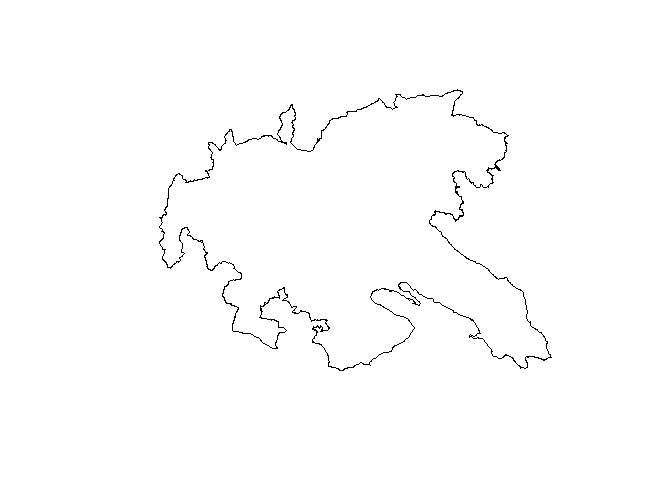
want all observations inside the polygon of the district of Constance
(Landkreis Konstanz, including Radolfzell… and a protected natural
area!) so I’ll first need to get it. For doing that I’ll use
osmdata::getbb, that uses the free Nominatim API provided by
Openstreetmap.
library("sf")
landkreis_konstanz <- osmdata::getbb("Landkreis Konstanz",
                             format_out = "sf_polygon")

plot(landkreis_konstanz)
Neither rebird nor spocc currently offer built-in trimming of
occurrence data to a polygon (whereas osmdata does). A further
difficulty created by eBird’s API is that it doesn’t allow for the use
of a bounding box, but instead demands a lat, lng and a dist
defining the radius of interest from given lat/lng in kilometers.
Thanks to Marco Sciaini for providing me
with an easy way to compute dist, using the sf package.
coord <- sf::st_coordinates(landkreis_konstanz)

bbox <- c(x1 = min(coord[, "X"]),
          x2 = max(coord[, "X"]),
          y1 = min(coord[, "Y"]),
          y2 = max(coord[, "Y"]))


center <- c(x = (bbox["x1"] + bbox["x2"])/2,
            y = (bbox["y1"] + bbox["y2"])/2)

dist <- landkreis_konstanz %>%
  sf::st_cast("POINT") %>%
  sf::st_distance() %>%
  max() * 0.5

dist
## 24129.15 m
Now, we can make the query.
birds <- rebird::ebirdgeo(species = NULL,
                          lng = center["x.x1"],
                          lat = center["y.y1"],
                          back = 30,
                          dist = as.numeric(
                            units::set_units(dist, "km")))
nrow(birds)
## [1] 55
str(birds)
## Classes 'tbl_df', 'tbl' and 'data.frame':    55 obs. of  12 variables:
##  $ lng            : num  8.94 8.94 8.94 8.94 8.94 ...
##  $ locName        : chr  "Radolfzeller Aachmündung (Bodensee)" "Radolfzeller Aachmündung (Bodensee)" "Radolfzeller Aachmündung (Bodensee)" "Radolfzeller Aachmündung (Bodensee)" ...
##  $ sciName        : chr  "Chroicocephalus ridibundus" "Motacilla alba" "Rallus aquaticus" "Aythya fuligula" ...
##  $ obsValid       : logi  TRUE TRUE TRUE TRUE TRUE TRUE ...
##  $ locationPrivate: logi  FALSE FALSE FALSE FALSE FALSE FALSE ...
##  $ obsDt          : chr  "2018-08-08 13:30" "2018-08-08 13:30" "2018-08-08 13:30" "2018-08-08 13:30" ...
##  $ obsReviewed    : logi  FALSE FALSE FALSE FALSE FALSE FALSE ...
##  $ comName        : chr  "Black-headed Gull" "White Wagtail" "Water Rail" "Tufted Duck" ...
##  $ lat            : num  47.7 47.7 47.7 47.7 47.7 ...
##  $ locID          : chr  "L3314048" "L3314048" "L3314048" "L3314048" ...
##  $ locId          : chr  "L3314048" "L3314048" "L3314048" "L3314048" ...
##  $ howMany        : int  NA 2 1 1 NA 3 NA NA 8 20 ...
Now that we have the occurrence data, let’s plot it to see whether trimming is required.
crs <- sf::st_crs(landkreis_konstanz)

birds_sf <- sf::st_as_sf(birds,
                         coords = c("lng", "lat"),
                         crs = crs)
library("ggplot2")
ggplot() +
  geom_sf(data = landkreis_konstanz) +
  geom_sf(data = birds_sf) +
  theme(legend.position = "bottom") +
  hrbrthemes::theme_ipsum() +
  ggtitle("eBird observations over the last 30 days",
          subtitle = "Observations within a circle around the County of Constance")
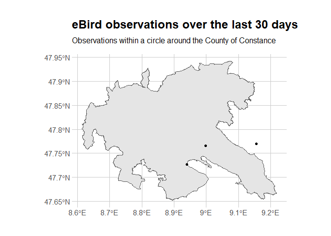
Yes, trimming is required! It’d have been too bad not to learn how to do it, anyway. We also add the MPI to the map.
# which parts of the oject are in the county
in_indices <- sf::st_within(birds_sf, landkreis_konstanz)

# filter them
trimmed_birds <- dplyr::filter(birds_sf,
                               lengths(in_indices) > 0)

# summarize to get no. of birds by  location
summarized_birds <- trimmed_birds %>%
  dplyr::group_by(locName) %>%
  dplyr::summarise(n = n())

# MPI
mpi <- opencage::opencage_forward("Am Obstberg 1 78315 Radolfzell",
                                  limit = 1)$results

coords <- data.frame(lon = mpi$geometry.lng,
                     lat = mpi$geometry.lat)

crs <- sf::st_crs(landkreis_konstanz)

mpi_sf <- sf::st_as_sf(coords,
                       coords = c("lon", "lat"),
                       crs = crs)

# Map!
ggplot() +
  geom_sf(data = landkreis_konstanz) +
  geom_sf(data = summarized_birds,
          aes(size = n), show.legend = "point") +
  hrbrthemes::theme_ipsum() +
  ggtitle("eBird observations over the last 30 days",
          subtitle = "County of Constance, MPI as a triangle") +
  geom_sf(data = mpi_sf,
          shape = 2)
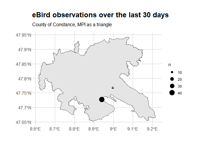
We got 49 observations (nrow(trimmed_birds)) of 49 species
(length(unique(trimmed_birds$comName))), over 2 places
(length(unique(trimmed_birds$locName))) during 5 observation sessions.
Hopefully merely an appetizer to what we can get from using the full
eBird dataset in the next section…
Note that the initial query could have been made with spocc which
would have helped using the rOpenSci occurrence suite.
birds2 <- spocc::occ(from = "ebird",
                     ebirdopts = list(method = "ebirdgeo",
                                      species = NULL,
                                      lng = center["x.x1"],
                                      lat = center["y.y1"],
                                      back = 30,
                                      dist = as.numeric(
                                        units::set_units(dist, "km"))))

mapr::map_leaflet(birds2)
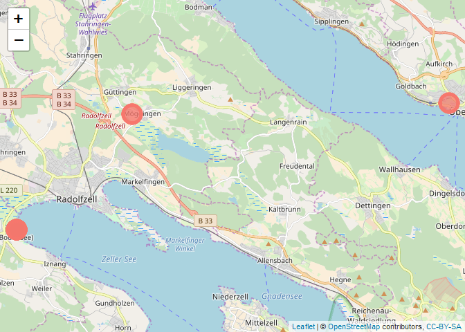
Quite handy!
Now, let’s explore the whole eBird dataset for Germany.
🔗 Using auk to process EBD dataset for Germany
After getting access to a custom dataset corresponding to the EBD for
Germany only, I used auk’s documentation and this
post to learn how to process
it. Since I wasn’t planning on zero-filling the data to get
presence/absence counts, I was able to ignore the sampling event data
that contains the checklist-level information (e.g. time and date,
location, and search effort information). For an example of a more
advanced auk workflow involving the full EBD, and sampling data,
refer to Matt Strimas-Mackey’s own blog post about his
package.
🔗 Preparing the dataset
Here, the workflow is to clean the data and to filter it using one
of auk’s built-in filters and then polygon filtering as earlier in
this post. All steps are quite fast, because the custom dataset for
Germany isn’t too big (a few hundred megabytes).
Cleaning happens in the following:
ebd_dir <- "C:/Users/Maelle/Documents/ropensci/ebird"

f <- file.path(ebd_dir, "ebd_DE_relMay-2018.txt")
f_clean <- file.path(ebd_dir, "ebd_DE_relMay-2018_clean.txt")
auk::auk_clean(f, f_out = f_clean, remove_text = TRUE)
Then one can filter the data. Note that the auk_extent function that
only retains observations within a bounding box has been renamed
auk_bbox in the dev version of auk, the old name will be deprecated
soon.
ebd_dir <- "C:/Users/Maelle/Documents/ropensci/ebird"
f_in_ebd <- file.path(ebd_dir, "ebd_DE_relMay-2018_clean.txt")

library("magrittr")
landkreis_konstanz_coords <- sf::st_coordinates(landkreis_konstanz)

ebd_filter <- auk::auk_ebd(f_in_ebd) %>%
  auk::auk_extent(c(min(landkreis_konstanz_coords[, "X"]),
                    min(landkreis_konstanz_coords[, "Y"]),
                    max(landkreis_konstanz_coords[, "X"]),
                    max(landkreis_konstanz_coords[, "Y"])))
ebd_filter
## Input
##   EBD: C:\Users\Maelle\Documents\ropensci\ebird\ebd_DE_relMay-2018_clean.txt
##
## Output
##   Filters not executed
##
## Filters
##   Species: all
##   Countries: all
##   States: all
##   BCRs: all
##   Spatial extent: Lon 8.6 - 9.2; Lat 47.7 - 47.9
##   Date: all
##   Start time: all
##   Last edited date: all
##   Protocol: all
##   Project code: all
##   Duration: all
##   Distance travelled: all
##   Records with breeding codes only: no
##   Complete checklists only: no
fs::dir_create("ebird")
f_out_ebd <- "ebird/ebd_lk_konstanz.txt"
f_out_sampling <- "ebird/ebd_lk_konstanz_sampling.txt"
ebd_filtered <- auk::auk_filter(ebd_filter, file = f_out_ebd,
                                overwrite = TRUE)
On top of this filtering with auk, after loading the data we filter
observations inside the polygon of the county.
crs <- sf::st_crs(landkreis_konstanz)

ebd <- auk::read_ebd(f_out_ebd) %>%
  sf::st_as_sf(coords = c("longitude", "latitude"),
                crs = crs)

in_indices <- sf::st_within(ebd, landkreis_konstanz)

ebd <- dplyr::filter(ebd, lengths(in_indices) > 0)

ebd <- as.data.frame(ebd)
🔗 What are the observed birds?
Before looking at species names, let’s have a brief look at the size and temporal extent of the data.
library("ggplot2")

dim(ebd)
## [1] 10156 41
ebd %>%
  dplyr::mutate(year = lubridate::year(observation_date)) %>%
ggplot() +
  geom_bar(aes(year))  +
  hrbrthemes::theme_ipsum(base_size = 12, axis_title_size = 12, axis_text_size = 12) +
  ylab("No. of eBird observations") +
  xlab("Time (years)") +
  ggtitle("Full eBird dataset for the County of Constance")
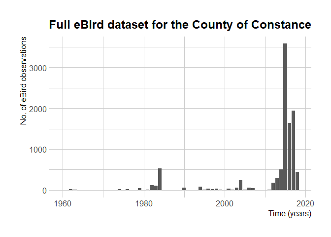
eBird started in 2002 but only became global in 2010. It allows people to enter older observations, though.
Now we can look at what birds have been reported the most.
ebd %>%
  dplyr::filter(approved) %>%
  dplyr::count(scientific_name, common_name) %>%
  dplyr::arrange(- n) %>%
  head(n = 10) %>%
  knitr::kable()
| scientific_name | common_name | n |
|---|---|---|
| Corvus corone | Carrion Crow | 288 |
| Turdus merula | Eurasian Blackbird | 285 |
| Anas platyrhynchos | Mallard | 273 |
| Fulica atra | Eurasian Coot | 268 |
| Parus major | Great Tit | 266 |
| Podiceps cristatus | Great Crested Grebe | 254 |
| Ardea cinerea | Gray Heron | 236 |
| Cygnus olor | Mute Swan | 234 |
| Cyanistes caeruleus | Eurasian Blue Tit | 233 |
| Chroicocephalus ridibundus | Black-headed Gull | 223 |
I had to google most of them, but only because I didn’t know the scientific and English names of these birds: they’re birds even I, not a birder, know, probably because they’re also common in Brittany where I grew up.
We can also look at birds whose observation was rejected. Out of 10156 observations only 64 were reviewed, and only 5 were not approved.
ebd %>%
  dplyr::select(scientific_name, common_name,
               approved, reviewed, reason) %>%
  dplyr::filter(!approved) %>%
  knitr::kable()
| scientific_name | common_name | approved | reviewed | reason |
|---|---|---|---|---|
| Cygnus atratus | Black Swan | FALSE | TRUE | Species-Introduced/Exotic |
| Cygnus atratus | Black Swan | FALSE | TRUE | Species-Introduced/Exotic |
| Cygnus atratus | Black Swan | FALSE | TRUE | Species-Introduced/Exotic |
| Oxyura leucocephala | White-headed Duck | FALSE | TRUE | Species-Introduced/Exotic |
| Mareca sibilatrix | Chiloe Wigeon | FALSE | TRUE | Species-Introduced/Exotic |
Black Swans are mostly present in Australia, imported and escaped in a few other places but eBird mostly doesn’t accept the entry of exotic species although it’s debated. In any case, eBird’s curation of the data entered is quite admirable.
🔗 Who observed birds?
In one of his latest blog posts Scott Chamberlain mentioned the legendary Lowell Ahart, super plant collector in Butte County, California. Does the county of Constance have a super birder?
(first_birder <- ebd %>%
  dplyr::count(observer_id) %>%
  dplyr::arrange(- n) %>%
  head(n = 1) )
## # A tibble: 1 x 2
##   observer_id     n
##   <chr>       <int>
## 1 obsr457108   3551
(proportion <- round(first_birder$n/nrow(ebd),
                    digits = 2))
## [1] 0.35
Wow, that person made 35% of eBird observations in the county! The EBD no longer provides names (consequence of the EU General Data Protection Regulation) but from the checklist ID one can get access to the checklist page e.g this one where the name of the observer is present. The super birder of the County of Constance is Antonio Anta Bink.
🔗 Conclusion
🔗 R packages for occurrence data
In this post I gave a rough view of what birds are present in the county around Radolfzell: Eurasian Blackbirds, Carrion Crows, Great Tits… but not Black Swans in eBird’s data. We mostly illustrated the use of two R packages accessing eBird’s data:
aukfor processing the gigantic whole eBird’s dataset.rebirdfor getting access to recent data via an API.rebirdis part of a larger collection of packages for occurrence data within rOpenSci’s suite, withspoccbeing an umbrella package accessing several data sources;scrubra helper for cleaning data obtained this way; andmapra utility package for mapping such data.
Explore these packages, and more of rOpenSci’s suite, by checking out our packages page!
🔗 More birding soon!
Stay tuned for the next post in this series, that’ll mark a break from modern data since we’ll try to extract information from old natural history bird drawings! After that, in a following post we’ll come back to the occurrence data obtained from eBird in order to complement it with open taxonomic and traits data. In the meantime, happy (e)birding!

