Parsing Metadata with R - A Package Story

Every R package has its story. Some packages are written by experts, some by novices. Some are developed quickly, others were long in the making. This is the story of jstor, a package which I developed during my time as a student of sociology, working in a research project on the scientific elite within sociology. Writing the package has taught me many things (more on that later) and it is deeply gratifying to see, that others find the package useful.

Before taking a look at the package’s inception however, I want to give you some basic information. JSTOR is a large archive for scientific texts, mainly known for their coverage of journal articles, although they recently added book chapters and other sources as well. They make all of their content available for researchers with their service Data for Research. With this data you can do text mining, citation analysis, and everything else you could come up with, using metadata and data about the content of the articles. The package I wrote, jstor, provides functions to import the metadata, and it has a few helper functions for common cleaning tasks. Everything you need to know about how to use it is on the package website. You will find three vignettes, with a general introduction, examples on how to import many files at once, and a few examples of known quirks of JSTORs data. There is also a lengthy case study that shows how to combine metadata and information on the articles’ content. If you still need more information, you can also watch my presentation at this year’s useR! in Brisbane or dive into the slides. But for now, let us turn back the clock to follow along my journey of developing the package.

🔗 Hacking Away

Back in March 2017, I was starting out as a MA-student of sociology in a research project concerned with the scientific elite within sociology and economics. The project had many goals but writing an R package was not one of them. At the start, I was presented with a dataset which was huge, at least for my terms: around 30GB of data, half of which was text, the other half 500,000 .xml-files. The dataset was incredible in its depth: we had all articles from JSTOR which belonged to the topics “sociology” and “economics”. To repeat: all articles that JSTOR has on those topics for all years JSTOR has data on.

My task was to somehow make this data accessible for our research. Since we are sociologists and no computer experts, and my knowledge of R was mainly self-taught, my approach was quite ad-hoc: “Let’s see, how we can extract relevant information for one file, and then maybe we can lapply over the whole set of files.” That is what the tidyverse philosophy and purrr tell you to do: solve it for one case using a function and apply this function to the whole set of files, cases, nested rows, or whatever. Long story short, you can do it like that, and I surely did it like that. But if I could start over and write a new version of the package, I would probably do a few things differently, one of which I discuss near the end of the post.

🔗 How (not) to import .xml-files

So, I had to start somewhere, and that was obviously importing the data into R. After searching and trying different packages, I settled on xml2::read_xml(). But then what. I had done a few pet projects with web-scraping but had no knowledge of XPATH-expressions and how to access certain parts of the document directly. 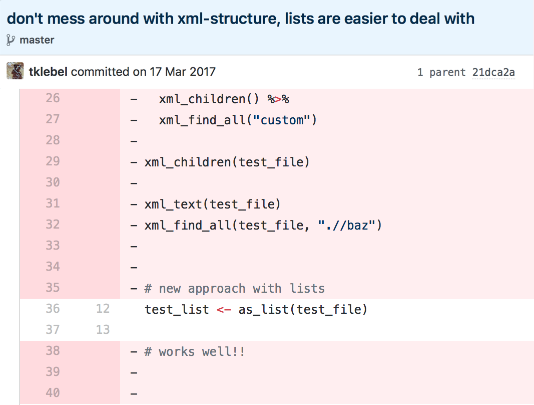After some stumbling around, I had found xml2::as_list() and was very happy: I could turn this unpleasant creature of XML into a pretty list, which I was accustomed to. My happiness is obvious when looking at the relevant commit message and the corresponding changes.

After turning the XML into a list, I would use something like listviewer::jsonedit() to inspect the elements, and extract what I needed. The approach was cumbersome, and the code was not pretty, since the original documents are deeply nested, and the structure was not always the same. But it worked, and I was happy with it, for the time being.

My functions looked something like this:

extract_contributors <- function(contributors) {
  if (is.null(contributors)) {
    return(NA)
  } else {
    contributors %>%
      map(extract_name) %>%
      bind_rows() %>%
      rename(given_names = `given-names`) %>%
      mutate(author_number = 1:n())
  }
}


find_meta <- function(meta_list) {
  front <- meta_list$front
  article <- front$`article-meta`

  # authors
  contributors <- article$`contrib-group`
  contributors <- extract_contributors(contributors)

  # piece together all elements
  data_frame(
    journal_id = front$`journal-meta`$`journal-id`[[1]],
    article_id = article$`article-id`[[1]],
    article_title = article$`title-group`$`article-title`[[1]],
    authors = list(contributors),
    article_pages = extract_pages(article)
  )
}

As you can see, there is a lot of indexing (like in journal_id = front$journal-meta$journal-id[[1]]) and mapping over lists.

The function would have been applied like so:

# one file
"file_path.xml" %>% 
  read_xml() %>% 
  as_list() %>% 
  find_meta()
  
# many files
c("mutliple.xml", "file.xml", "paths.xml") %>% 
  map(read_xml) %>% 
  map(as_list) %>% 
  map(find_meta)

As can be expected when parsing deeply nested lists which do not always have the same structure, this quickly escalated into more and more complex and sometimes quite ridiculous functions:

extract_name <- function(x) {
  x %>%
    flatten() %>%
    flatten() %>%
    flatten() %>%
    .[!(names(.) %in% c("x", "addr-line"))] %>%
    as_data_frame()
}

But, as I said, I was solving problems with the tools I already knew, so I was happy.

🔗 Benchmarking my code

At some point though, I started benchmarking my solutions. I experimented with mclapply and it doubled the speed of execution on my machine, but it was still very slow: Parsing the content after importing and transforming it into a list took 7.2 seconds for 3,000 files. For 200,000 files of sociological articles this would amount to 8 hours. And importing and converting to a list took a lot of time too. Although I didn’t think at that time, that I would need to import the files more than once or at most twice (which I had to do later to update results after we got new versions with better data), I decided that this was too slow, and I looked for better options.

The first idea which I had was simply to scale computing power: I had a faster machine at home and planned to read the data into R at work, save it as .rds, and then process it at home on the faster machine (for some reason I didn’t want to carry the original data home). Apparently, this is not as easy as it sounds. If you parse a file with xml2::read_xml() you don’t get the content of the file, but only an object that points to the file, and you can then extract content with xml_child() and other functions. But you cannot use readr::write_rds to save the file, instead you need xml2::xml_serialize() and xml2::xml_unserialize() and they require an open connection, and so on. I can tell you that, since Jim Hester kindly responded to my question on StackOverflow. He had a further hint:

[…] I would seriously consider using XPATH expressions to extract the desired data, even if you have to rewrite code. […] Xpath extracting just the elements you are interested in is going to run much faster than converting the entire data to a list first then manipulating that. ~Jim Hester

And this is what I did. Just for the fun of it, I benchmarked two versions: my function before re-writing to using XPATH expressions, and the function today. The current version is a lot safer and handles many edge-cases, but it is still around 5 times faster. Furthermore, the processing time depends less on how complex the original file is, and more on how much information is being read. With the new version of the function, around 30% of the time is spent on reading the file from disk, while the remaining 70% deal with parsing the content. In contrast, the old version spent around 85% of the time on parsing the file.

microbenchmark::microbenchmark(
  convert = jst_example("sample_with_references.xml") %>% 
    read_xml() %>% 
    as_list(),
    
  old = jst_example("sample_with_references.xml") %>% 
    read_xml() %>% 
    as_list() %>% 
    find_meta(),
  
  new = jst_get_article(jst_example("sample_with_references.xml"))
)

## Unit: milliseconds
##     expr       min        lq     mean    median       uq       max neval
##  convert 35.621488 39.274647 44.29424 43.530006 46.64541 114.12766   100
##      old 42.038368 46.596185 51.49769 49.711072 52.43276 134.12999   100
##      new  8.675674  9.054154 10.33858  9.365577 10.16726  23.88457   100

I uploaded the old code to a gist: old_functions.R. If you want to run the benchmark on your own, execute the following snippet first:

# load current functions
library(jstor)

# load old function
devtools::source_gist(
  "https://gist.github.com/tklebel/11d2664ac2bc754ddc367369eec1a660",
  filename = "old_functions.R"
)

library(tidyverse)
library(xml2)

🔗 Doing It Properly

🔗 Working with XPATH-expressions

Rewriting my functions was not that much of a hassle, in the end. I had turned my functions into a package early on and had already included many test cases with testthat to make sure everything works as expected. This helped a lot for re-structuring the code, since I already knew what my output should look like, and I only had to change the intermediate steps.

The work on re-writing progressed quickly. The first step was to simply extract the identifier for the journal within which the article was published:

find_meta <- function(xml_file) {
  if (identical("xml_document" %in% class(xml_file), FALSE)) {
    stop("Input must be a `xml_document`", call. = FALSE)
  }

  front <- xml_find_all(xml_file, "front")

  data_frame(
    journal_id = extract_jcode(front)
  )
}


extract_jcode <- function(front) {
  front %>%
    xml_child("journal-meta") %>%
    xml_find_first("journal-id") %>%
    xml_text()
}

I quickly added new parts, although it didn’t feel all too easy: I basically had to learn how to navigate within the document via XPATH.

Another thing I took up during this re-write was regularly benchmarking my functions. Since I lacked the technical expertise to know up front which approach would be faster, I benchmarked possibilities to figure it out. The following benchmark compares three versions of extracting the text from the node named volume. Especially the first two seemed very similar to me and it was not at all obvious, which one would be faster.

test_file <- jst_example("sample_with_references.xml") %>% xml2::read_xml()

fun1 <- function() {
  xml_find_all(test_file, "front/.//volume/.//text()") %>% as.character()
}
fun2 <- function() {
  xml_find_all(test_file, "front/.//volume") %>% xml_text()
}
fun3 <- function() {
  xml_find_all(test_file, "front") %>%
    xml_child("article-meta") %>%
    xml_child("volume") %>%
    xml_text()
}
  
# `bench::mark` checks if results are consistent, which is usually a good thing 
# to do
bench::mark(fun1(), fun2(), fun3(), min_time = 2)

# A tibble: 3 x 14
  expression   min  mean median    max `itr/sec` mem_alloc  n_gc n_itr total_time
  <chr>      <bch> <bch> <bch:> <bch:>     <dbl> <bch:byt> <dbl> <int>   <bch:tm>
1 fun1()     254µs 332µs  286µs 53.4ms     3011.    12.7KB    15  5757      1.91s
2 fun2()     230µs 295µs  262µs 48.6ms     3393.    10.2KB    14  6518      1.92s
3 fun3()     663µs 838µs  764µs 54.7ms     1193.    35.2KB    16  2254      1.89s
# ... with 4 more variables: result <list>, memory <list>, time <list>, gc <list>

Although the unit is microseconds here, the difference between fun2 and fun3 is quite substantial, if you want to do it 500,000 times: 4.2 minutes^[For this calculation I am taking the difference in the medians from the benchmark. The difference is about 502 microseconds. If we multiply this by 500,000 and then divide it by 1,000,000 (1 microsecond equals 1/1,000,000 seconds), we get 251 seconds, which is close to 4 minutes (251/60 = 4.18)]) . If you have to extract multiple elements from a file (which I was doing), then this quickly adds up. What is the reason for this big difference? I’d guess that fun2 is fastest since it only calls two functions, and not four, and because xml_text() probably converts the content directly to character in C++, which is faster than calling as.character afterwards. Still, I am not a computer scientist, so I am not entirely sure about that.

🔗 Using profvis to find bottlenecks

After rewriting and expanding the functionality, I was still not happy, however, since the code was slower than I thought it should be. At this point, I dug deeper again, using the package profvis to find bottlenecks. Oddly enough, I had introduced a bottleneck right at the beginning: I was using data_frame (which is equivalent to tibble()) to create the object my function would return. Unfortunately, tibble (and data.frame as well) are quite complex functions. They do type checking and other things, and if you do this repeatedly, it quickly adds up.

You can see the difference yourself:

microbenchmark::microbenchmark(
  tibble = tibble::tibble(a = rnorm(10), b = letters[1:10]),
  new_tibble = tibble::new_tibble(list(a = rnorm(10), b = letters[1:10]))
)

## Unit: microseconds
##        expr     min       lq     mean   median      uq      max neval
##      tibble 332.902 479.7430 624.1354 621.7795 716.437 1944.658   100
##  new_tibble  76.833 106.5485 155.4881 151.2890 172.570  974.428   100

The difference is not huge (~4 minutes for 500,000 documents^[The calculation is similar as above: (624.1354 - 151.2890) * 5e+05 / 1e+06 / 60 = 3.94 minutes.]), but my actual layout was a lot more complex, since it was using nested structures in a weird way:

# dummy data
authors <- tibble::tribble(
  ~first_name, ~last_name, ~author_number,
  "Pierre",    "Bourdieu", 1,
  "Max",       "Weber",    2,
  "Karl",      "Marx",     3
)

# this approach made sense to me, since the data structure was indeed nested,
# and it seemed similar to the approach of mutate + map + unnest.
old_approach <- function(authors) {
  res <- tibble::data_frame(id = "1",
                            authors = list(authors))
  
  tidyr::unnest(res, authors)
}

# this is obviously a lot simpler
new_approach <- function(authors) {
  data.frame(id = "1",
             authors = authors)
}


microbenchmark::microbenchmark(
  old = old_approach(authors),
  new = new_approach(authors)
)

## Unit: microseconds
##  expr      min       lq      mean   median       uq      max neval
##   old 3973.088 4168.759 5195.9013 4615.224 5617.265 12761.89   100
##   new  246.695  266.216  586.4228  316.517  356.386 22031.18   100

The difference is significant, amounting to around 36 minutes more for 500,000 documents^[The calculation is similar as above: (4615.224 - 316.517) * 5e+05 / 1e+06 / 60 = 35.82 minutes.], if I would have kept the old version.

Unfortunately, using profvis for such small and fast functions does not work well out of the box:

profvis::profvis({
  old_approach()
})

#> Error in parse_rprof(prof_output, expr_source) : No parsing data available. 
#> Maybe your function was too fast?

A simple solution is to rerun the function many times. Note, however, that this does not increase reliability and reproducibility of the results. The function is not measured 500 times, the result being the mean or median (like in microbenchmark), but it is simply the aggregate of running the function 500 times. This can vary quite a bit. All in all, though, I found it still useful to judge if any part of the code is orders of magnitude slower than the rest.

In the following chunk I define the function again for two reasons: first to separate all computations into separate lines. This ensures, that we get a measurement for each line. Second, the code needs to be supplied either within the call to profvis, or it must be defined in a sourced file, otherwise the output will not be as informative, because profvis will not be able to access the functions’ source code.

profvis::profvis({
  
  old_approach <- function(authors) {
    res <- tibble::data_frame(id = "1",
                              authors = list(authors))
    
    tidyr::unnest(res, authors)
  }

  purrr::rerun(500, old_approach(authors))
})

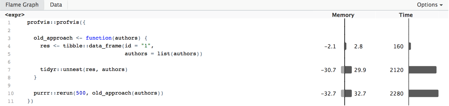
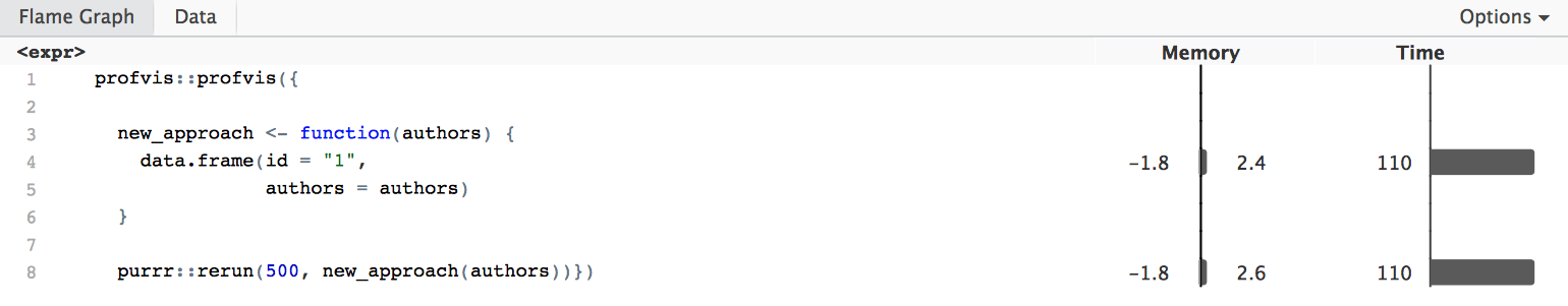
We can see that the call to tidyr::unnest takes up a lot of time, thus it would be good to get rid of it. The new approach does not need unnesting, and is roughly 17 times faster:

profvis::profvis({

  new_approach <- function(authors) {
    data.frame(id = "1",
               authors = authors)
  }
  
  purrr::rerun(500, new_approach(authors))})

In the end, by assessing the efficiency of functions repeatedly and optimising several parts, I was able to trim down execution time considerably overall. For 25,000 files, which is the maximum number of files you can receive at one time through the standard interface of JSTOR/DfR, execution time is slightly under 4 minutes, or 2 minutes if executed in parallel (at least on my machine with a 2,8GHz Intel i5).

🔗 Lessons learned

I have learned many things while working on this package. While I acquired certain skills (like writing simple XPATH-queries), I want to highlight a few general things.

Something which is probably true for many people working with and developing for R, is that community is important. Without the efforts of many others, through paid work or by spending their time voluntarily, developing the package would not have been possible. This is true for the many packages my code builds on, for the suite of packages that helps in developing and maintaining packages, for answers I got over StackOverflow, and last but not least for the helpful comments I received by Elin Waring and Jason Becker during the review process for onboarding the package.

A lesson which is more or less obvious from what I wrote above would be to benchmark your code, if you are planning on running it often. Packages like microbenchmark, profvis or bench can help you in different ways to make sure that your code runs more efficiently.

At the beginning of the post I mentioned, that there might be a better approach on parsing those files altogether. Before I finish, I want to briefly elaborate on that thought.

The general approach I took when writing the package was inspired by the idea of functional programming, that can be implemented in R through lapply or similar functions within the purrr-package. The approach is to write a function that solves your problem for one case, and then to apply it to all cases. In my case, this leads to some duplication and inefficiency: The package has several functions that extract certain parts of the metadata-files. This makes sense, since you only might be interested in certain parts, and parsing everything else would be a waste of time. Unfortunately, if you happen to be interested in two parts all the time, this means that each function has to read the original file separately. There is no economy of scales, so to speak, because the file is read again for each part which is to be extracted. An alternative would have been to write a general wrapper function that reads in the files and then applies each function in turn. I suspect that this would be quite complex, given that the code should also be able to run in parallel in a proper way. This, and the fact that I already spent a lot of time writing the package, mean that I will most likely not add improvements on this side. There are however many other options for improvement, and I will gladly point you to a few of them.

🔗 Options to contribute

I have strived for a proper test coverage, and I’d say it is decent at 91%. There are a few cases where adding coverage would not be too difficult, which I have mentioned in issue #71. Another area where there is still some work to do is extracting a few more fields from the documents. This would involve some XPATH but could be a good starting point if you are curious about how this works. The corresponding issues are #23 and #32. Any help, even fixing typos in the vignettes or documentation, is greatly appreciated, so if you want to get into contributing to a package, just go for it! I will try to help you with any hiccups along the way.