The Antarctic/Southern Ocean rOpenSci community

🔗 Antarctic/Southern Ocean science and rOpenSci

Collaboration and reproducibility are fundamental to Antarctic and Southern Ocean science, and the value of data to Antarctic science has long been promoted. The Antarctic Treaty (which came into force in 1961) included the provision that scientific observations and results from Antarctica should be openly shared. The high cost and difficulty of acquisition means that data tend to be re-used for different studies once collected. Further, there are many common data requirement themes (e.g. sea ice information is useful to a wide range of activities, from voyage planning through to ecosystem modelling). Support for Antarctic data management is well established. The SCAR-COMNAP Joint Committee on Antarctic Data Management was established in 1997 and remains active as a SCAR Standing Commitee today.

Software development to support Antarctic data usage is growing, but still lags behind the available data, and some common tasks are still more difficult than we would like. Starting in late 2017, the Scientific Committee on Antarctic Research has been collaborating with rOpenSci to strengthen the Antarctic and Southern Ocean R/science communities. Our focus is on data and tasks that are common or even unique to Antarctic and Southern Ocean science, including supporting the development of R packages to meet Antarctic science needs, guides for R users and developers, active fora for open discussions, and strengthening connections with the broader science world.

🔗 First steps in building the community

Our initial efforts have focused on two things:

1. compiling a list of existing resources likely to be useful to the community: see the task view. This document outlines some relevant packages, including some that are under active development.
2. improving core functionality centred around three key tasks that many researchers find problematic:
   • getting hold of data. The physical environment is important to a large cross-section of Antarctic science, and environmental data often come from satellite, model, or similar sources,
   • processing those data to suit particular study interests, such as subsetting or merging with field or other data,
   • producing maps for exploratory analyses or publications.

A couple of packages have been formally peer-reviewed and onboarded into rOpenSci, with others in development. Example usage of a few of these packages is demonstrated below.

🔗 Get involved

Please get involved!

• contribute your Antarctic R knowledge, your Antarctic use case for a package, or ask a question in the dedicated Antarctic and Southern Ocean category of rOpenSci’s discussion forum,

• make a suggestion — perhaps for Antarctic-related functionality that you feel is missing from the current R ecosystem?

• contribute an Antarctic R package, or improve the documentation or code of an existing one. See the task view as a starting point,

• join the #antarctic rOpenSci Slack channel for R users and developers — contact us at [email protected] for an invitation to join. Slack is a great space in which to have conversations with the rOpenSci community, or to give us feedback in a less-public manner,

• participate in the broader rOpenSci community. Follow on Twitter, read the blog, and check out the ecosystem of R packages.

The administrative contacts for this initiative are Ben Raymond, Sara Labrousse, Michael Sumner, and Jess Melbourne-Thomas. Contact us via [email protected], or find us on Slack or Twitter.

🔗 Demo

A lightning trip through the land of bowerbird, raadtools, SOmap, and antanym. First install some packages, if needed.

## make sure we have the packages we need
req <- setdiff(c("dplyr", "ggplot2", "remotes"), installed.packages()[, 1])
if (length(req) > 0) install.packages(req)

## and some github packages
req <- c("ropensci/antanym", "AustralianAntarcticDivision/blueant",
         "AustralianAntarcticDivision/raadtools",
         "AustralianAntarcticDivision/SOmap")
req <- req[!basename(req) %in% installed.packages()[, 1]]
if (length(req) > 0) remotes::install_github(req)

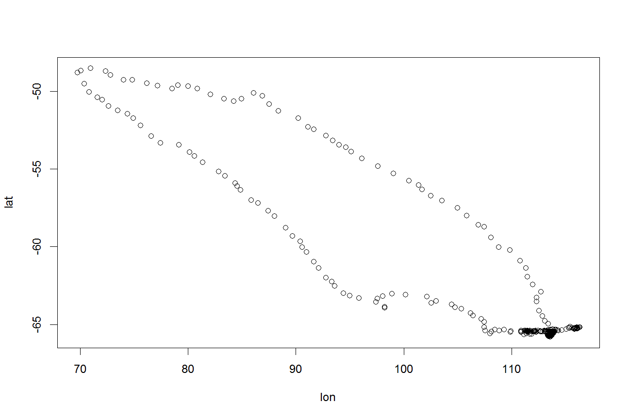
Let’s say that we have some points of interest in the Southern Ocean — perhaps a ship track, or some stations where we took marine samples, or as we’ll use here, the track of an elephant seal as it moves from the Kerguelen Islands to Antarctica and back again (Data from IMOS 2018¹, provided as part of the SOmap package).

library(dplyr)
library(ggplot2)

data("SOmap_data", package = "SOmap")
ele <- SOmap_data$mirounga_leonina %>% dplyr::filter(id == "ct96-05-13")
with(ele, plot(lon, lat))

🔗 Fetching our environmental data

Very commonly, we want to know about the environmental conditions at our points of interest. For the remote and vast Southern Ocean these data typically come from satellite or model sources. Some data centres provide extraction tools that will pull out a subset of data to suit your requirements, but often it makes more sense to cache entire data collections locally first and then work with them from there.

bowerbird provides a framework for downloading data files to a local collection, and keeping it up to date. The companion blueant package provides a suite of definitions for Southern Ocean and Antarctic data sources that can be used with bowerbird. It encompasses data such as sea ice, bathymetry and land topography, oceanography, and atmospheric reanalysis and weather predictions, from providers such as NASA, NOAA, Copernicus, NSIDC, and Ifremer.

Why might you want to maintain local copies of entire data sets, instead of just fetching subsets of data from providers as needed?

• many analyses make use of data from a variety of providers (in which case there may not be dynamic extraction tools for all of them),
• analyses might need to crunch through a whole collection of data in order to calculate appropriate statistics (temperature anomalies with respect to a long-term mean, for example),
• different parts of the same data set are used in different analyses, in which case making one copy of the whole thing may be easier to manage than having different subsets for different projects,
• a common suite of data are routinely used by a local research community, in which case it makes more sense to keep a local copy for everyone to use, rather than multiple copies being downloaded by different individuals.

In these cases, maintaining local copies of a range of data from third-party providers can be extremely beneficial, especially if that collection is hosted with a fast connection to local compute resources (virtual machines or high-performance computational facilities).

Install the package if needed:

library(remotes)
install_github("AustralianAntarcticDivision/blueant")

To use blueant, we first choose a location to store our data. Normally this would be a persistent location (perhaps on shared storage if multiple users are to have access to it), but for the purposes of demonstration we’ll just use a temporary directory here:

my_data_dir <- tempdir()

We’ll focus on two sources of environmental data: sea ice and water depth. Note that water depth does not change with time but sea ice is highly dynamic, so we will want to know what the ice conditions are like on a day-to-day basis.

Download daily sea ice data (from 2013 only), and the ETOPO2 bathymetric data set. ETOPO2 is somewhat dated and low resolution compared to more recent data, but will do as a small dataset for demo purposes:

library(blueant)
src <- bind_rows(
    sources("NSIDC SMMR-SSM/I Nasateam sea ice concentration", hemisphere = "south",
            time_resolutions = "day", years = 2013),
    sources("ETOPO2 bathymetry"))
result <- bb_get(src, local_file_root = my_data_dir, clobber = 0, verbose = TRUE,
                 confirm = NULL)

##  
## Sat Nov 10 01:00:48 2018 
## Synchronizing dataset: NSIDC SMMR-SSM/I Nasateam sea ice concentration 
##  
##  [... output truncated]

Now we have local copies of those data files. The sync can be run daily so that the local collection is always up to date - it will only download new files, or files that have changed since the last download. For more information on bowerbird, see the package vignette.

Details of the files can be found in the result object, and those files could now be read with packages such as raster. However, we are collecting data from a range of sources, and so they will be different in terms of their grids, resolutions, projections, and variable-naming conventions, which tends to complicate these operations. In the next section we’ll look at the raadtools package, which provides a set of tools for doing common operations on these types of data.

🔗 Using those environmental data: raadtools

raadtools is suite of functions that provide consistent access to a range of environmental and similar data, and tools for working with them. It is designed to work data collections maintained by the bowerbird/blueant packages.

Load the package and tell it where our data collection has been stored:

library(raadtools)
set_data_roots(my_data_dir)

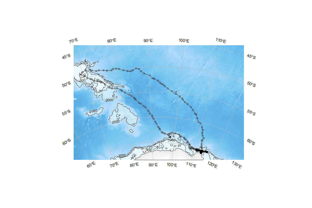
Define our spatial region of interest and extract the bathymetry data from this region, using the ETOPO2 files we just downloaded:

roi <- round(c(range(ele$lon), range(ele$lat)) + c(-2, 2, -2, 2))
bx <- readtopo("etopo2", xylim = roi)

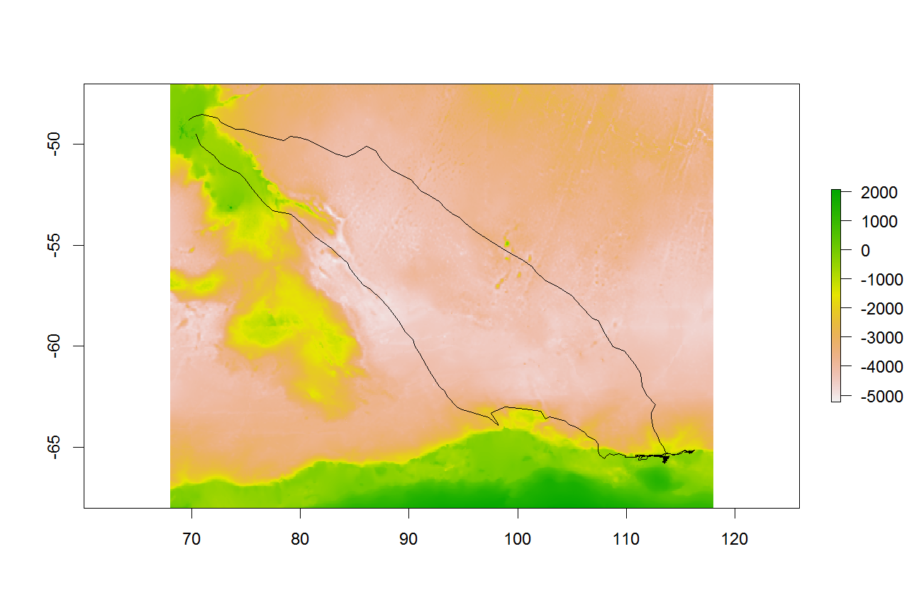
And now we can make a simple plot of our our track superimposed on the bathymetry:

plot(bx)
lines(ele$lon, ele$lat)

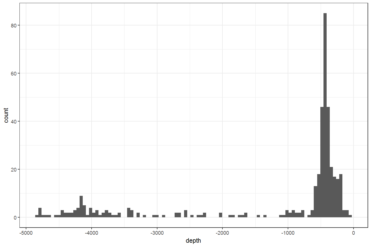
We can also extract the depth values along our track using the extract() function in raadtools:

ele$depth <- extract(readtopo, ele[, c("lon", "lat")], topo = "etopo2")

Plot the histogram of depth values, showing that most of the track points are located in relatively shallow waters:

ggplot(ele, aes(depth)) + geom_histogram(bins = 100) + theme_bw()

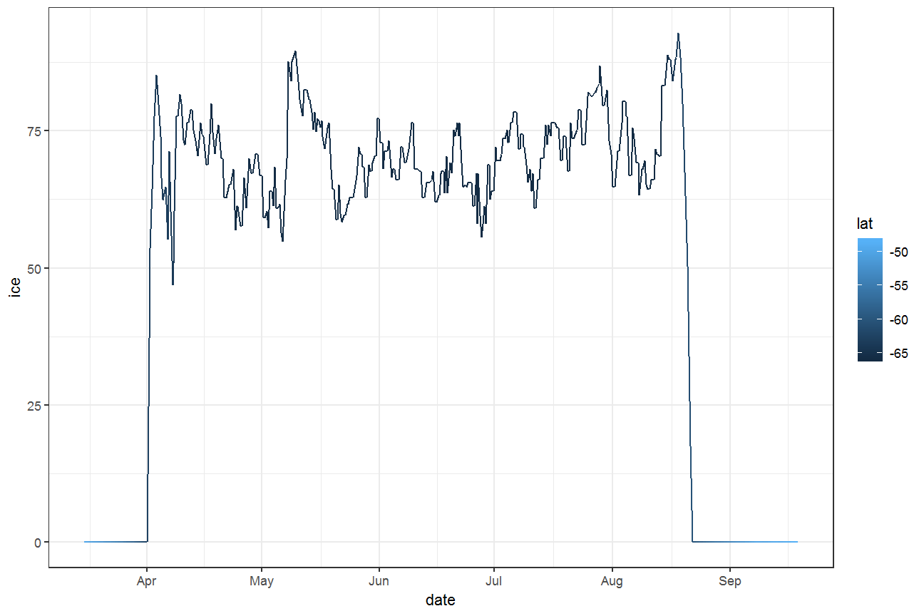
This type of extraction will also work with time-varying data — for example, we can extract the sea-ice conditions along our track, based on each track point’s location and time:

ele$ice <- extract(readice, ele[, c("lon", "lat", "date")])
## points outside the ice grid will have missing ice values, so fill them with zeros
ele$ice[is.na(ele$ice)] <- 0
ggplot(ele, aes(date, ice, colour = lat)) + geom_path() + theme_bw()

Or a fancy animated plot, using gganimate (code not shown for brevity, but you can find it in the page source). The hypnotic blue line shows the edge of the sea ice as it grows over the winter season, and the orange is our elephant seal:

🔗 Mapping

Creating maps is another very common requirement, and in the Southern Ocean this brings a few challenges (e.g. dealing with the dateline when using polar-stereographic or similar circumpolar projections). There are also spatial features that many users want to show (coastlines, oceanic fronts, extent of sea ice, place names, etc). The in-development SOmap package aims to help with this.

library(SOmap)
SOauto_map(ele$lon, ele$lat, mask = FALSE)

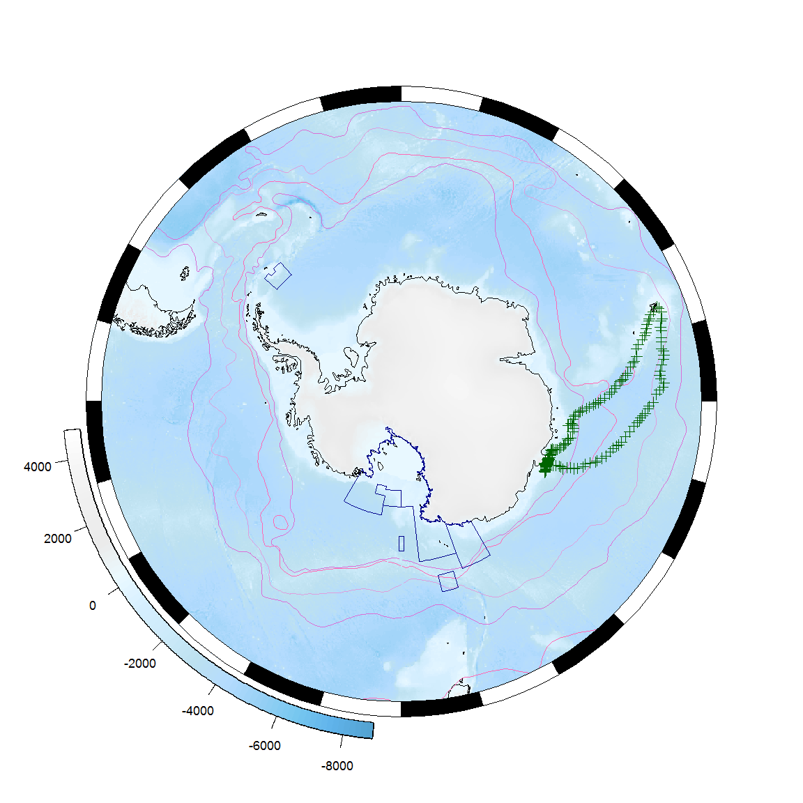
Or a full-hemisphere map:

## first transform our track to polar-stereographic coordinates
library(sp)
library(raster)
ele_sp <- ele
coordinates(ele_sp) <- c("lon", "lat")
projection(ele_sp) <- "+proj=longlat +ellps=WGS84"
ele_sp <- spTransform(ele_sp,
            CRS("+proj=stere +lat_0=-90 +lat_ts=-71 +lon_0=0 +k=1 +x_0=0 +y_0=0 
            +datum=WGS84 +units=m +no_defs +ellps=WGS84 +towgs84=0,0,0"))

## plot the base map with ocean fronts shown
SOmap(fronts = TRUE)
## add current marine protected areas
SOmanagement(MPA = TRUE, mpacol = "darkblue")
## add our track
plot(ele_sp, col = "darkgreen", add = TRUE)

🔗 Place names

SCAR maintains a gazetteer of place names in the Antarctic and surrounding Southern Ocean², which is available to R users via the antanym package:

library(antanym)

## The Composite Gazetteer of Antarctica is made available under a CC-BY license.
## If you use it, please cite it:
## Composite Gazetteer of Antarctica, Scientific Committee on Antarctic Research.
##   GCMD Metadata (https://data.aad.gov.au/aadc/gaz/scar/)

xn <- an_read(cache = "session", sp = TRUE)

There is no single naming authority for place names in Antarctica, and so there can be multiple names for a single feature (where it has been given a name by more than one country). We can trim our names list down to one name per feature (here, preferentially choosing the UK name if there is one):

xn <- an_preferred(xn, origin = "United Kingdom")

How many place names do we have?

nrow(xn)

## [1] 19742

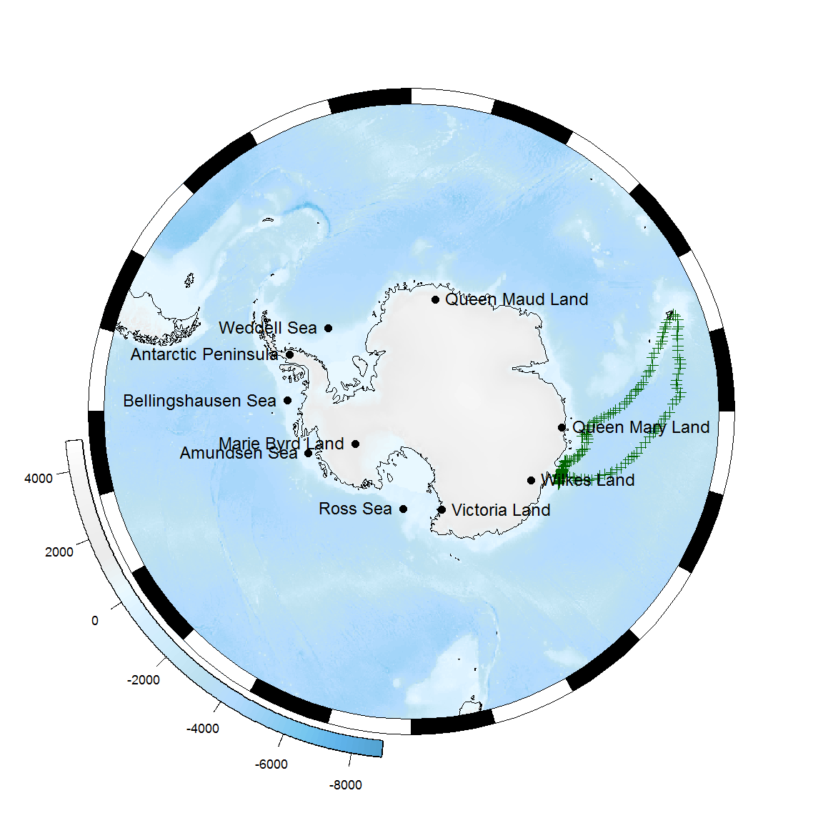
OK, we can’t show all of these — which ones would be best to show on this map? Let’s ask antanym for suggestions:

xns <- an_suggest(xn, map_scale = 20e6, map_extent = c(-180, 180, -90, -40))

## transform to our map projection and take the first 10 names
xns <- as_tibble(spTransform(xns, projection(Bathy))) %>% head(10)

## add them to the map
SOmap()
plot(ele_sp, col = "darkgreen", add = TRUE)
with(xns, points(x = longitude, y= latitude, pch = 16))
with(xns, text(x = longitude, y= latitude, labels = place_name,
               pos = 2 + 2*(longitude > 0)))

🔗 Next steps

There is plenty more that these and other R packages can do for Antarctic and Southern Ocean science. See the package READMEs and vignettes for more examples, keep an eye out for future developments … and get involved!

🔗 References