Co-localization analysis of fluorescence microscopy images

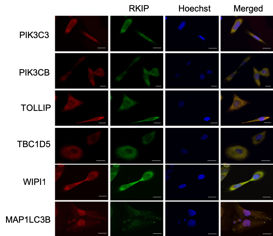
A few months ago, I wasn’t sure what to expect when looking at fluorescence microscopy images in published papers. I looked at the accompanying graph to understand the data or the point the authors were trying to make. Often, the graph represents one or more measures of the so-called co-localization, but I couldn’t figure out how to interpret them. It turned out; reading the images is simple. Cells are simultaneously stained by two dyes (say, red and green) for two different proteins. The color turns yellow in the merged image when the two proteins localize in proximity.

A recent publication from our laboratory included microscopy images and a quantification graph. The standard analysis protocol is to use ImageJ with a specialized plug-in for the co-localization analysis such as coloc2 or Fiji. The images were processed one at a time; subtracting the background, selecting regions of interest and calculating the co-localization statistics. This work was done manually and repeated with minor changes in the parameters each time. At the end, there was no way to make this process reproducible, and we included only the final output in an otherwise fully reproducible article.

For those two specific reasons; the need for manual work and the lack of reproducibility, I thought it would be great if I could do this analysis in R. There are several R packages for image processing such as EBImage, imager and magick. These packages provided the functionality needed for conducting this analysis. So I put the pieces together in an R package to simplify this analysis for my future self and for others who might find it useful. This is colocr, a simple R package for conducting co-localization analysis of fluorescence microscopy images. In particular, it semi-automates the selections of regions of interest-arguably the most time-consuming step- and comes with a Shiny app for visually comparing the outputs of different parameters before writing a final script.

🔗 How would have we done it differently?

In this recent article I referred to earlier, we assessed the co-localization of several proteins with RKIP (Raf-kinas inhibitor protein) in DU145 prostate cancer cell line. For each of these proteins, we generated multiple frames, a hundred in total. We then processed the images one by one and repeated the process with each minor change in the parameters. Now we can use colocr, in just a few lines of code, to apply the same analysis.

A selection of the images were presented in the article in a similar figure.

We can calculate the Pearson’s Correlation Coefficients (PCC) of multiple images at once using the following chunk of code.

## load required libraries
library(tidyverse)
library(colocr)

# load images
fls <- list.files('images', pattern = '*.jpg', recursive = TRUE)

# apply co-localization test
tst <- image_load(fls) %>%
  roi_select(threshold = 90, n = 3) %>%
  roi_test()

And the results can be visualized in a graph.

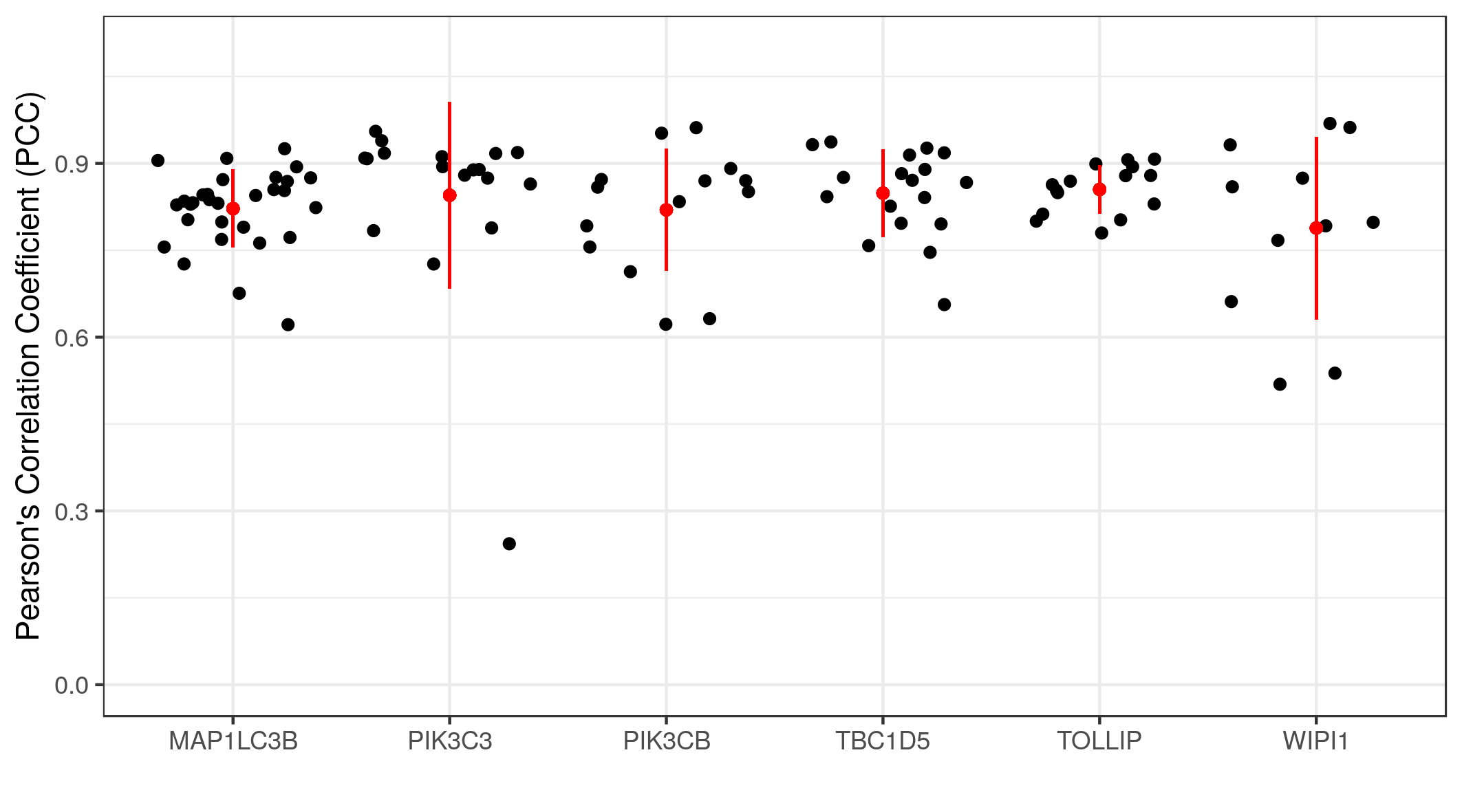
The graph shows the co-localization statistics (PCC) for RKIP and six other proteins (x-axis). The pixel intensity of the channel of each protein (red) and RKIP (green) in three regions of interest from multiple images were used to calculate the PCC. In all cases, the correlations were above 0.75 with reasonable variance. This means a high degree of co-localization between RKIP and the six target proteins.

The following code is to generate the graph.

## load required libraries
library(tidyverse)

# make the graph of calculated correlations
names(tst) <- str_split(fls, pattern = '/', simplify = TRUE)[, 1]

bind_rows(tst, .id = 'protein') %>%
  group_by(protein) %>%
  mutate(ave = mean(pcc),
         sd = sd(pcc),
         upper = ave + sd,
         lower = ave - sd) %>%
  ggplot(aes(x = protein, y = pcc)) +
  geom_jitter() +
  geom_point(aes(y = ave), color = 'red') +
  geom_linerange(aes(ymax = upper, ymin = lower), color = 'red') +
  lims(y = c(0, 1.1)) +
  labs(x = '', y = "Pearson's Correlation Coefficient (PCC)") +
  theme_bw()

While developing colocr, I focused on breaking down the steps of the analysis into intuitive pieces. Hopefully, in a way that the potential user, or “myself in a few months”, can understand easily. By keeping the number of the functions limited, the inputs and the outputs consistent and making things visual as much as possible, I hope using the package needs less investment by the user. I hope biologists who are not familiar with R can still find this work useful. One thing helped me organize and iterate on the code. This was developing a Shiny app as an interface to the package.

🔗 Developing a Shiny app in an R package

At first, I thought of adding a Shiny app as an extra feature for users who might need it. I quickly realized that for this use case, selecting regions of interest might require trial-and-error on the side of the user to arrive at suitable parameters for the selection. Having to develop the app forced me to think about organizing the functions, their input and output in a certain way. Namely, mapping the functions to the steps of the analysis that the user has to think about and making visual output a priority. Finally, testing the app exposed errors in the intermediates which might have been buried in otherwise seemingly fine R objects. Overall, I learned a thing or two about writing Shiny apps to go with R packages when possible even if it won’t make the cut in the release.

• I found it useful to work on the app as early as possible and improving it side by side with the core functionality. As explained earlier, this helped me to think about the inputs and the output from a user’s perspective.
• I learnt to isolate the source code for the app from that of the package functions as much as possible. One may host the app code in a separate repository and include it in the project as a git submodule. Some might find this necessary, but I found it easier this way to keep track of the changes in the app and testing it on Travis.

🔗 Submitting R packages for reviewing by rOpenSci

colocr was my second submission to rOpenSci. My first submission was a package called cRegulome. In both cases, I had positive experiences. So I would like to thank the rOpenSci editor, the reviewers (Hao Zhu, Sean Hughes) and Jeroen Ooms who helped us to resolve issues related to running the package on Windows. At a risk of an understatement, here are three benefits I got from submitting my packages to rOpenSci which others might find encouraging doing the same.

• Reviewing the source could at an early stage help to spot mistakes and introducing improvement to the code that might escape the authors themselves.
• Often the editor and the reviewers are experts in R and the subject matter, so they can offer ideas and suggestion to improve the design of the package. Adding to being an early test users who provided useful insights.
• Writing and distributing code might not be everyone’s strongest skill. And certain aspects of it might be challenging. The rOpenSci team provide support during the process I found encouraging.

🔗 Things to improve

I am working on improving the performance and adding more features. I welcome all contributions. Two areas of improvement are

• Change dependency from imager to magick to take advantage of the well tested magick classes and functionality. issue #4.

• Add a feature to allow for adjusting for artifacts in the images such as luminescence, which might affect the final calculations. issue #5.

🔗 Other resources

• colocr source code on GitHub, here
• The Shiny app, here
• The package vignette, here