
Tuesday, January 22, 2019 From rOpenSci (https://ropensci.org/blog/2019/01/22/waterinfo-tidal-eel/). Except where otherwise noted, content on this site is licensed under the CC-BY license.
Do you know what that sound is, Highness? Those are the Shrieking Eels — if you don’t believe me, just wait. They always grow louder when they’re about to feed on human flesh. If you swim back now, I promise, no harm will come to you. I doubt you will get such an offer from the Eels.
Vizzini, The Princess Bride
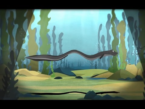
European eels (Anguilla anguilla) have it tough. Not only are they depicted as monsters in movies, they are critically endangered in real life. One of the many aspects that is contributing to their decline is the reduced connectivity between their freshwater and marine habitats. Eels are catadromous: they live in freshwater, but migrate to the Sargasso Sea to spawn, a route that is blocked by numerous human structures (shipping locks, sluices, pumping stations, etc.). Pieterjan Verhelst studies the impact of these structures on the behaviour of eels, making use of the fish acoustic receiver network that was established as part of the Belgian LifeWatch observatory. This animated video gives a quick introduction to his research and the receiver network:
In this blog post, we’ll explore if the migration of one eel is influenced by the tide. It’s a research use case for our R package wateRinfo, which was recently peer reviewed (thanks to reviewer Laura DeCicco and editor Karthik Ram for their constructive feedback!) and accepted as a community-contributed package to rOpenSci.
🔗 Meet Princess Buttercup
Pieterjan provided us the tracking data for eel with transmitter A69-1601-52622. Let’s call her Princess Buttercup, after the princess that almost got eaten by the Shrieking Eels in the classic and immensly quotable movie The Princess Bride.
eel <- read_csv(here("data", "eel_track.csv"))
Her tracking data consists of the residence time interval (arrival until departure) at each receiver station that detected her along the Scheldt river. It also contains the calculated residencetime (in seconds), as well as the station name, latitude and longitude.
| date | receiver | latitude | longitude | station | arrival | departure | residencetime |
|---|---|---|---|---|---|---|---|
| 2016-10-19 | VR2W-112297 | 51.00164 | 3.85695 | s-Wetteren | 2016-10-19 23:44:00 | 2016-10-19 23:48:00 | 240 |
| 2016-10-19 | VR2W-112287 | 51.00588 | 3.77876 | s-2 | 2016-10-19 16:07:00 | 2016-10-19 19:12:00 | 11100 |
| 2016-10-20 | VR2W-122322 | 51.02032 | 3.96965 | s-2a | 2016-10-20 13:18:00 | 2016-10-20 13:23:00 | 300 |
| 2016-10-20 | VR2W-122322 | 51.02032 | 3.96965 | s-2a | 2016-10-20 02:21:00 | 2016-10-20 02:29:00 | 480 |
| 2016-10-20 | VR2W-115438 | 51.01680 | 3.92527 | s-Wichelen | 2016-10-20 01:01:00 | 2016-10-20 01:09:00 | 480 |
| 2016-10-20 | VR2W-122322 | 51.02032 | 3.96965 | s-2a | 2016-10-20 05:52:00 | 2016-10-20 06:00:00 | 480 |
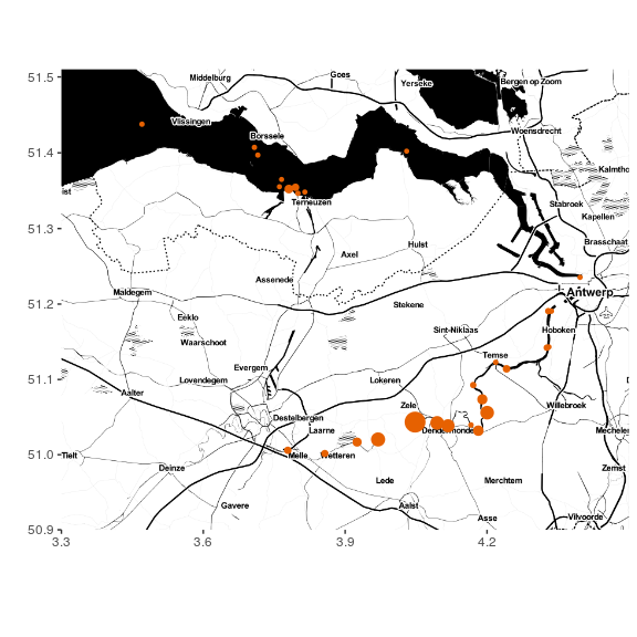
Using the latitude, longitude and total residencetime for each station, we can map where Princess Buttercup likes to hang out:
🔗 Moving up and down the Scheldt river
To get a better sense of her journey along the river, we add a distance_to_sea (in meters) for the stations, by joining the tracking data with a distance reference file 1. We can now plot her movement over time and distance:
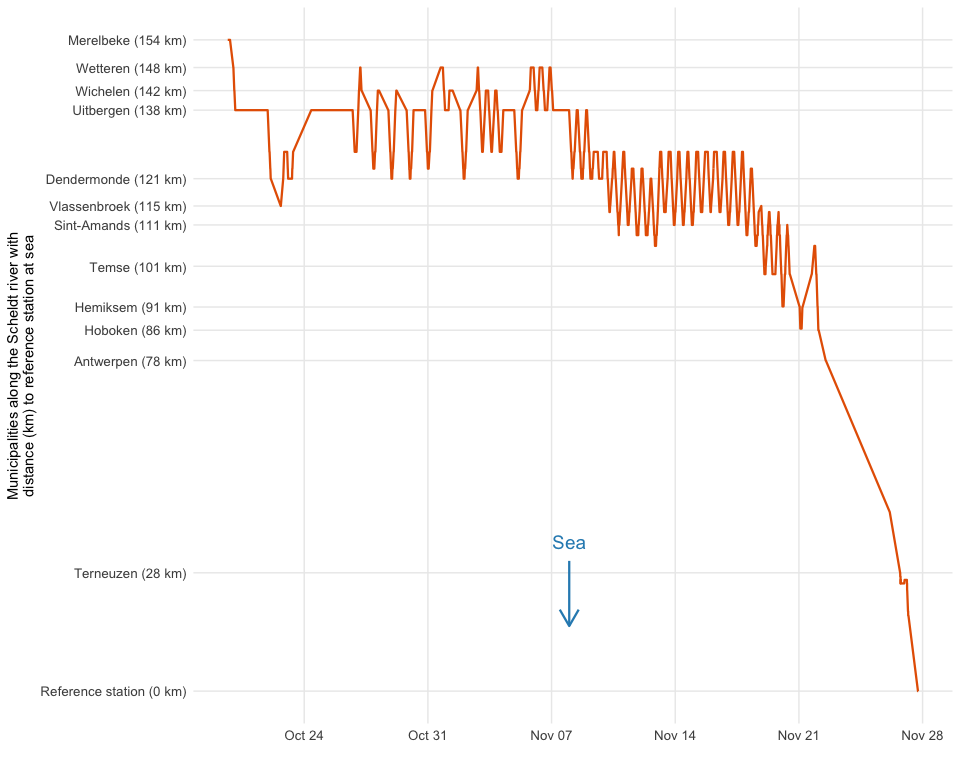
Princess Buttercup’s signal was picked up by receivers in Merelbeke (near Ghent) shortly after she was captured and released there on October 11. She resided in a 40 km stretch of the river (between Wetteren and Sint-Amands) for about a month before migrating towards the sea and starting the long journey towards the Sargasso Sea. The periodic movement pattern up and down the river during the second half of November is of particular interest: it looks like tidal frequency 2. It would be interesting to compare the movement pattern with real water level data from the Scheldt river… which is where our wateRinfo package comes in.
🔗
Getting tidal data with the wateRinfo package
Waterinfo.be, managed by the Flanders Environment Agency (VMM) and Flanders Hydraulics Research, is a website where one can find real-time water and weather related environmental variables for Flanders (Belgium), such as rainfall, air pressure, discharge, and water level. The website also provides an API to download time series of these measurements as open data, but compositing the download URL with the proper system codes can be challenging. To facilitate users in searching for stations and variables, subsequently downloading data of interest and incorporating waterinfo.be data access in repeatable workflows, we developed the R package wateRinfo to do just that. See the package documentation for more information on how to install and get started with the package.
Timeseries in waterinfo.be (identified by a ts_id) are a combination of a variable, location (station_id) and measurement frequency (15min by default). For example:
library(wateRinfo)
get_stations("water_level") %>%
  select(ts_id, station_id, station_name, parametertype_name) %>%
  head()
| ts_id | station_id | station_name | parametertype_name |
|---|---|---|---|
| 92956042 | 39483 | Kieldrecht/Noordzuidverbinding | H |
| 31683042 | 21995 | Leuven/Dijle1e arm/stuw K3 | H |
| 20682042 | 20301 | StMichiels/Kerkebeek/Rooster | H |
| 96495042 | 10413 | Oudenburg/Magdalenakreek | H |
| 25074042 | 20788 | Schulen/Inlaat A/WB_Schulensbroek | H |
| 2006042 | 10432 | Merkem/Steenbeek | H |
At the time of writing (see this issue), the stations measuring water levels in the Scheldt tidal zone are not yet included by the API under the core variable water_level and are thus not yet available via get_stations("water_level"). We therefore rely on a precompiled list of tidal time series identifiers (tidal_zone_ts_ids):
tidal_zone_ts_ids <- read_csv(here("data", "tidal_zone_ts_ids.csv"))
From which we select the 10-min frequency tidal timeseries in the Scheldt river:
| ts_id | station_id | station_name | portal_bekken |
|---|---|---|---|
| 55419010 | 0430087 | Sint-Amands tij/Zeeschelde | Beneden-Scheldebekken |
| 55565010 | 0430029 | Tielrode tij/Durme | Beneden-Scheldebekken |
| 55493010 | 0430081 | Temse tij/Zeeschelde | Beneden-Scheldebekken |
| 54186010 | 0419418 | Dendermonde tij/Zeeschelde | Beneden-Scheldebekken |
| 54493010 | 0430078 | Hemiksem tij/Zeeschelde | Beneden-Scheldebekken |
| 55355010 | 0430091 | Schoonaarde tij/Zeeschelde | Beneden-Scheldebekken |
| 53989010 | 0419484 | Antwerpen tij/Zeeschelde | Beneden-Scheldebekken |
| 54606010 | 0430071 | Kallosluis tij/Zeeschelde | Beneden-Scheldebekken |
| 56088010 | 0430062 | Prosperpolder tij/Zeeschelde | Beneden-Scheldebekken |
| 54936010 | 0430068 | Liefkenshoek tij/Zeeschelde | Beneden-Scheldebekken |
| 55059010 | 0430242 | Melle tij/Zeeschelde | Beneden-Scheldebekken |
This wateRinfo vignette shows how to download data for multiple stations at once using wateRinfo and dplyr. We use a similar approach, but instead of manually providing the start and end date, we get these from Princess Buttercup’s tracking data:
tidal_data <-
  tidal_zone_ts_ids %>%
  group_by(ts_id) %>%

  # Download tidal data for each ts_id (time series id)
  do(get_timeseries_tsid(
      .$ts_id,
      from = min(eel$date), # Start of eel tracking data
      to = max(eel$date),   # End of eel tracking data
      datasource = 4
  )) %>%

  # Join data back with tidal_zone_ts_id metadata
  ungroup() %>%
  left_join(tidal_zone_ts_ids, by = "ts_id")
In just a few lines of code, we downloaded the tidal data for each measurement station for the required time period. 👌
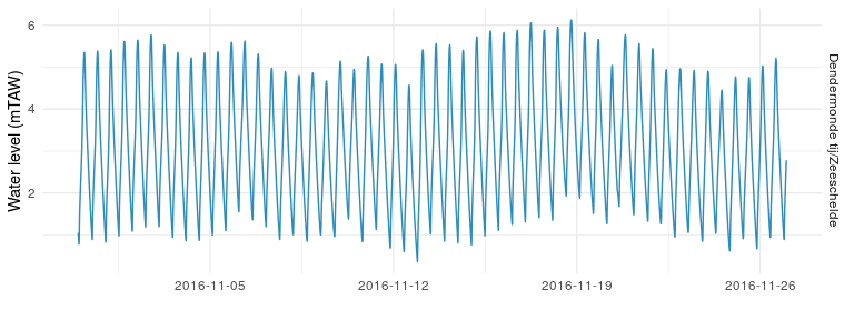
The water level is expressed in mTAW (meter above mean sea level) 3. Let’s plot the data for a station (here Dendermonde in November 2016) to have a look:
We now have all the pieces to verify if Princess Buttercup was surfing the tide back and forth.
🔗 Is Princess Buttercup surfing the tide?
Let’s add the tidal data to Princess Buttercup’s journey plot we created before. The first step is to join the tidal data with the same distance reference file to know the distance from each tidal station to the sea:
tidal_data <-
  tidal_data %>%
  left_join(
    distance_from_sea %>% select(station, distance_from_sea, municipality),
    by = c("station_name" = "station")
  ) %>%
  filter(station_name != "Hemiksem tij/Zeeschelde") # Exclude (probably erroneous) data from Hemiksem
To avoid visual clutter, we’ll use ridges (from ggridges) to display the tidal data for each station over time:
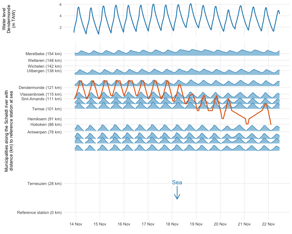
Looking at the plot, Princess Buttercup seems to be “lazy” and drift with the tide. Rising water levels push her upstream, while decreasing water levels bring her closer to sea again. On November 22 (see also previous plot), she embarks on her migration for real.
🔗 Conclusion
In this blogpost we used the wateRinfo package to gain some insight in the movement/migration behaviour of an individual eel. We hope the package can support many more research questions and that you have fun storming the castle.
- For a more in depth study of eel migration behaviour in response to the tide, see Verhelst et al. (2018).
- For more info on the package, see the package website.
- For the full code of this blogpost, see this repository.
🔗 Acknowledgements
Waterinfo.be data is made available by the Flanders Environment Agency, Flanders Hydraulics Research, Agentschap Maritieme Dienstverlening & Kust and De Vlaamse Waterweg. The fish acoustic receiver network, as well as the work by Stijn and Peter, is funded by FWO as part of the Flemish contribution to LifeWatch. The animated video on eel research was funded by the Flanders Marine Institute (VLIZ), coordinated by Karen Rappé and Pieterjan Verhelst, animated by Steve Bridger, and narrated by Bryan Kopta.
If you want to get in touch with our team, contact us via Twitter or email.
To represent the data along a straight line (y-axis), we calculated the distance along the river from each station to a reference station close to the sea (
ws-TRAWL), using acostDistancefunction. See this script for more the details on the calculation. ↩︎The Scheldt is under tidal influence from its river mouth all the way to Ghent (160km upstream) where it is stopped by sluices. The tide goes much further than the freshwater-saltwater boundary of the river. ↩︎
TAW means Tweede Algemene Waterpassing, a reference height for Belgium. ↩︎
Filed under
Suggest an edit
Open a pull request
