
Thursday, November 14, 2019 From rOpenSci (https://ropensci.org/blog/2019/11/14/workloopr-release/). Except where otherwise noted, content on this site is licensed under the CC-BY license.
Studies of muscle physiology often rely on closed-source, proprietary software for not only recording data but also for data wrangling and analyses. Although specialized software might be necessary to record data from highly-specialized equipment, data wrangling and analyses should be free from this constraint. It’s becoming more common for researchers to provide code along with published papers (but usually as Matlab scripts…ugh), but it is still typical for most analyses to be performed with code that stays in-house. Even worse is when some of the steps are carried out in a non-reproducible way, like needing to click and drag sliders across a screen (by hand!!) to select a data range of interest.
To give muscle physiologists a set of tools to help perform reproducible research, we present our new R package workloopR.
🔗 What it does
workloopR (pronounced “work looper”) provides a variety of features that we hope will help the typical muscle physiology researcher’s workflow. These include:
- Data import from
.ddffiles, like those produced by Aurora Scientific1, with retention of important metadata like file creation times and stimulus protocols. - Data import from non-
ddffiles through an object constructor (vignette here!) - Automatic cycle selection within data, with three options for how cycles are defined; see our
select_cycles()function and some tips here - Gear ratio correction and other forms of transformation; see Data transformation functions
- Work loop analyses, which integrate muscle force and length change to determine mechanical work output (and power output)
- Analyses of twitch and tetanic data to determine the time course of force production
And the ability to do all of the above in batch (i.e., import, wrangle, and analyze all data files within a directory) and then summarize the major results. Vignette here!
For more info, along with a variety of vignettes that give examples with code, check out our documentation site. We recommend starting with the Introductory vignette.
🔗 Some perks of using workloopR
🔗 Metadata
One thing we think is helpful to researchers is how workloopR automatically retains metadata when reading a .ddf file. We’ll demonstrate with the example work loop file provided with the package; first, let’s load the package and import some data.
library(workloopR)

## import the workloop.ddf file included within workloopR
wl_dat <-read_ddf(system.file("extdata", "workloop.ddf",
                              package = 'workloopR'),
                  phase_from_peak = TRUE)
Important metadata from the file are stored as attributes of the object. Here’s what’s stored for the work loop file:
names(attributes(wl_dat))
##  [1] "names"              "class"              "row.names"
##  [4] "stimulus_frequency" "cycle_frequency"    "total_cycles"
##  [7] "cycle_def"          "amplitude"          "phase"
## [10] "position_inverted"  "units"              "sample_frequency"
## [13] "header"             "units_table"        "protocol_table"
## [16] "stim_table"         "stimulus_pulses"    "stimulus_offset"
## [19] "stimulus_width"     "gear_ratio"         "file_id"
## [22] "mtime"
Specific metadata can be called via either attributes() or attr(). For example, we’ll take a look at the stimulus protocol, which shows the specific pattern of electrical stimulation that was delivered to the muscle during the experiment:
attr(wl_dat,"stim_table")
##   offset frequency width pulses cycle_frequency
## 1  0.012       300   0.2      4              28
## 2  0.000         0   0.0      0               0
There’s lots of useful info here: offset refers to the span of time (usually in secs) that elapsed before the stimulation began; frequency and width give info on how often (in Hz) and for how long (ms) the muscle was stimulated; pulses shows the total number of stimulus pulses that were delivered; and cycle_frequency shows the frequency (Hz) of muscle length oscillation for further context.
🔗 Visualization
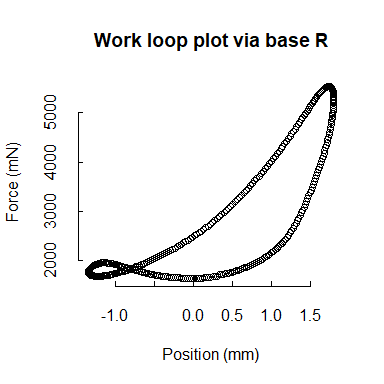
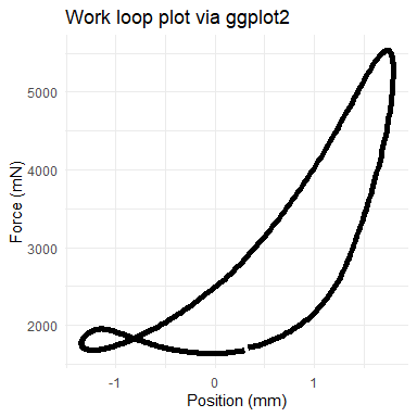
Although our functions do not generate plots, each is designed to be friendly to either base R or ggplot2 (and other Tidyverse packages). For example, we’ll show a work loop plotted in two ways. Because mechanical work is the product of force (y-axis) and distance (“Position” here, x-axis), the area within the loops of the following plots corresponds to the work that is performed by the muscle.
library(ggplot2)

## select cycles 3 through 5 using a l0-to-l0 definition
wl_selected <- select_cycles(wl_dat, cycle_def = "lo", keep_cycles = 3:5)

## apply a gear ratio correction, run the analysis function,
## and then get the full object
wl_analyzed <- analyze_workloop(wl_selected, GR = 2)

## base R work loop plot for the second retained cycle (cycle "b")
plot(wl_analyzed$cycle_b$Position,
     wl_analyzed$cycle_b$Force,
     xlab = "Position (mm)",
     ylab = "Force (mN)",
     main = "Work loop plot via base R",
     bty = "n", tck = 0.02)

## now via ggplot
 ggplot(wl_analyzed$cycle_b, aes(x = Position, y = Force)) +
  geom_path(lwd = 2) +
  labs(y = "Force (mN)", x = "Position (mm)") +
  ggtitle("Work loop plot via ggplot2") +
  theme_minimal()
See our Plotting vignette for more plotting ideas.
🔗 Summarizing a set of trials
The batch processing capabilities of workloopR should also be handy for efficiently analyzing all files within a specific folder, e.g., a set of trials from a single experiment. Here’s an example:
## batch read and analyze a set of work loop trials stored within one directory
wl_batch_analyzed <- read_analyze_wl_dir(
                        system.file("extdata/wl_duration_trials",
                                    package = 'workloopR'),
                        sort_by = 'file_id',
                        phase_from_peak = TRUE,
                        cycle_def = 'lo',
                        GR = 2,
                        keep_cycles = 3
                     )

## now create a summary of the trials
wl_batch_summarized <- summarize_wl_trials(wl_batch_analyzed)
wl_batch_summarized
##         File_ID Cycle_Frequency Amplitude  Phase Stimulus_Pulses
## 1 01_4pulse.ddf              28     1.575 -24.36               4
## 2 02_2pulse.ddf              28     1.575 -24.64               2
## 3 03_6pulse.ddf              28     1.575 -24.92               6
## 4 04_4pulse.ddf              28     1.575 -24.64               4
##   Stimulus_Frequency      mtime     Mean_Work  Mean_Power
## 1                300 1572459771  0.0027387056 0.078427135
## 2                300 1572459771  0.0009849216 0.027832717
## 3                300 1572459771 -0.0002192395 0.004323004
## 4                300 1572459771  0.0022793831 0.065468837
For more, see our Batch processing vignette.
🔗 How to get workloopR
We are not (yet) on CRAN but the package is available through rOpenSci’s GitHub:
#install.packages("devtools") # if devtools is not installed
devtools::install_github("ropensci/workloopR")

## To build vignettes as well:
devtools::install_github("ropensci/workloopR", build_vignettes = TRUE)
🔗 Feel free to make suggestions or requests
workloopR, as the name implies, was originally designed to handle data from work loop experiments as well as experiments that are complementary to work loops like twitch and tetanic trials.
We are happy to expand the scope of the package to incorporate even more types of analyses of muscle physiology or biomechanics. We’re presently eager to add data import functions for non-ddf file types. We’re also interested in integrating support for electromyographic (EMG) data recorded directly from muscles, but that may take a little longer to develop.
Should you like to suggest a specific feature, please use the Issues page of our repository.
🔗 Package review by rOpenSci and JOSS
We are thankful for the suggestions we’ve already received. workloopR benefited a lot from peer review of code through rOpenSci. Special thanks to Julia Romanowska (jromanowska) and Eric Brown (eebrown) for reviewing our code and giving helpful suggestions on how to improve the clarity of workloopR’s presentation.
We are also happy to share that a journal article that accompanies this package was also peer reviewed and accepted by the Journal of Open Source Software (JOSS)2.
🐢
Software from Aurora Scientific: https://aurorascientific.com/products/muscle-physiology/muscle-software/ ↩︎
Baliga V. and Senthivasan S (2019). workloopR: Analysis of work loops and other data from muscle physiology experiments in R. Journal of Open Source Software, 4(43), 1856, https://doi.org/10.21105/joss.01856 ↩︎
Filed under
Suggest an edit
Open a pull request
