
Tuesday, November 10, 2020 From rOpenSci (https://ropensci.org/blog/2020/11/10/coronaviruses-and-hosts/). Except where otherwise noted, content on this site is licensed under the CC-BY license.
Emerging viruses might be on everyone’s mind right now, but as an epidemiologist and disease ecologist I’ve always been interested in how and why pathogens move from animal hosts to humans. The current pandemic of the disease we call COVID-19 is caused by Severe acute respiratory syndrome (SARS) coronavirus 2 (SARS-CoV-2), a virus that has emerged from wildlife like SARS coronavirus and Middle East respiratory syndrome (MERS) coronavirus did previously. Although these viruses are now widely known, there are many more coronaviruses out there in nature, many of which we know little about.
There’s perhaps no better time to dive into understanding where viruses like these originate. Genome sequence repositories represent a wealthy source of data to understand the diversity of viruses and their relationships with their hosts. However, the sheer volume of data and lack of standardisation for some features can make it challenging to use these repositories in practice. In this post, I’ll demonstrate the use of the rentrez and taxizedb packages to search, retrieve and resolve information about genetic sequences of coronaviruses and their animal hosts - and ask which host species have the most coronavirus sequences been sampled from? Here’s a high-level summary of the functions we’ll use.
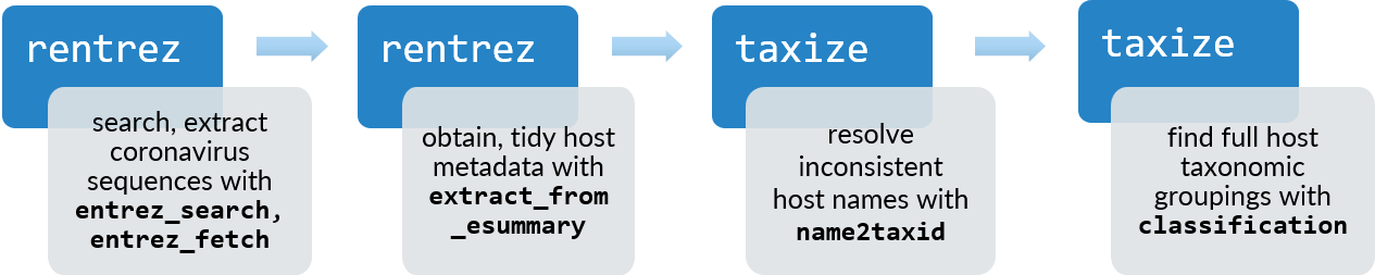
Flow diagram of functions used in each package to identify hosts associated with coronavirus sequences
I’ll focus on NCBI’s GenBank1, an open-access repository where sequences are submitted and described by individual users. We can look at the exponential rise in viral genome sequences by importing the release dates of those indexed by NCBI’s Genome Reports and plotting a cumulative curve.
library(dplyr)
library(ggplot2)
library(magrittr) # load magrittr for use of the pipe operator (%>%)

genbank_seqs <- read.table("ftp://ftp.ncbi.nlm.nih.gov/genomes/GENOME_REPORTS/viruses.txt",
sep = "\t", header = TRUE, comment.char = "!", quote = "", fill = TRUE)

monthly_seqs <- genbank_seqs$Release.Date %>%
  as.Date(format="%Y/%m/%d") %>%
  cut("month") %>%
  table() %>%
  as.data.frame() %>%
  rename(month = ".", total = Freq) %>%
  mutate(month = as.Date(month), total = cumsum(total))

ggplot(monthly_seqs, aes(month, total)) +
  geom_line(lwd=1.4) +
  xlab('Year') +
  ylab("Number of virus genome sequences") +
  scale_x_date(limits = as.Date(c('2000-01-01',Sys.Date()))) +
  theme_bw()
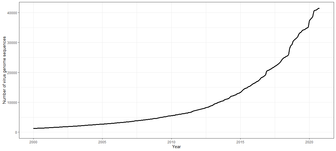
Viral genome sequence availability between 2000 and present
If we were interested in a small set of viruses, for example if we wanted to construct a specific phylogeny, we might reasonably be able to select and filter these genome sequences manually through web interfaces. In fact, a powerful new interface of the NCBI Virus front-end to GenBank was unveiled for this purpose earlier this year. However, if we want to investigate broader viral diversity (or use a data-hungry method like neural networks), we’d benefit from a more reproducible, automated approach.
🔗 Obtaining virus sequences with rentrez
🔗 Searching sequences
rentrez2 is a package by David Winter designed to interface with various NCBI databases (collectively known as entrez), including GenBank.
As such, it can not only conduct search requests in a single database, but also cross-reference them (see the vignette for some nice examples of this).
For now let’s simply try and find whether there are sequences available for Pangolin coronavirus in GenBank’s nucleotide sequence database (i.e., db ="nuccore").
This virus recently received a lot of attention because its spike protein (which is thought to be important in determining host range) is very similar to that of SARS-CoV-23,4.
We can use entrez_search() to conduct a general search across all fields.
library(rentrez)
pang_cov_ids <- entrez_search(db="nuccore", term="Pangolin coronavirus")
Registered S3 method overwritten by 'httr':
  method           from
  print.cache_info hoardr
pang_cov_ids
Entrez search result with 14 hits (object contains 14 IDs and no web_history object)
 Search term (as translated):  "Pangolin coronavirus"[Organism] OR Pangolin coron ...
Looks like there are 14 available genome sequences for this virus -
note that this query doesn’t return the actual sequences, but the specific entry IDs.
If we want to directly retrieve sequences, we can use entrez_fetch(), referencing these Pangolin coronavirus IDs.
Here I’ve set rettype to output the sequences in FASTA format, a standard bioinformatics format readable by many other packages/software.
pang_cov_seqs <- entrez_fetch(db="nuccore", id = pang_cov_ids$ids, rettype = "fasta_cds_na")
# trim the FASTA string to show first protein coding nucleotide sequence as an example
gsub("\n\n.*", "", pang_cov_seqs)
[1] ">lcl|MT799526.1_cds_QLR06869.1_1 [gene=S] [protein=surface glycoprotein] [protein_id=QLR06869.1] [location=1..3798] [gbkey=CDS]\nATGTTGTTTTTCTTCTTTTTACACTTTGCCTTAGTAAATTCACAATGTGTTAATTTAACAGGTAGAGCTG\nCTATCCAGCCTTCATTCACCAATTCCTCTCAAAGAGGTGTTTATTATCCTGACACCATATTTAGATCAAA\nCACACTTGTGTTGAGTCAGGGTTACTTTTTACCTTTTTATTCTAATGTTAGCTGGTATTATGCATTGACA\nAAAACTAACAGTGCTGAAAAGAGAGTTGATAACCCTGTTTTGGATTTCAAAGACGGTATTTACTTTGCTG\nCAACTGAAAAATCTAACATTGTCAGAGGTTGGATCTTTGGAACGACTCTTGACAACACATCACAGTCACT\nTTTGATAGTTAACAACGCAACTAATGTTATCATCAAAGTTTGTAATTTCCAGTTTTGTTATGACCCTTAC\nCTTAGTGGTTATTATCATAACAATAAAACGTGGAGCACGAGAGAGTTTGCTGTTTATTCCTCTTATGCCA\nATTGCACTTTTGAGTATGTGTCTAAGTCTTTTATGCTAGATATAGCTGGCAAAAGTGGCTTATTTGACAC\nATTAAGAGAGTTTGTTTTCCGAAATGTCGACGGATATTTCAAGATTTACTCAAAATACACACCTGTTAAT\nGTAAATAGTAATTTACCTATAGGTTTTTCAGCACTTGAACCTCTTGTTGAAATTCCAGCTGGCATAAATA\nTTACTAAATTTAGAACACTCCTCACTATACATAGAGGAGACCCCATGCCTAATAATGGCTGGACAGTCTT\nTTCAGCTGCTTATTACGTGGGCTATTTAGCTCCACGTACATTTATGTTAAATTATAATGAAAATGGTACA\nATAACAGATGCTGTTGATTGTGCCCTAGATCCTCTATCTGAGGCTAAATGCACATTAAAATCCTTAACTG\nTTGAAAAAGGAATCTATCAGACTTCTAACTTTAGAGTTCAACCAACTGAATCTATAGTTAGGTTTCCAAA\nTATTACAAACTTATGCCCTTTTGGTGAAGTTTTCAATGCAACCACTTTTGCATCTGTTTATGCTTGGAAT\nAGAAAGAGAATCAGTAACTGTGTTGCTGATTACTCTGTTCTTTACAACTCCACTTCTTTCTCAACATTCA\nAATGTTATGGAGTTTCACCAACCAAACTAAATGATCTCTGCTTTACTAACGTTTATGCAGACTCATTTGT\nAGTTAGAGGTGATGAAGTCAGACAAATTGCTCCAGGACAAACAGGAAGAATTGCTGACTATAATTATAAA\nCTCCCTGATGATTTCACAGGTTGTGTAATAGCTTGGAATTCTAACAACCTTGATTCTAAGGTTGGTGGTA\nATTATAACTACCTTTATAGATTGTTTAGAAAGTCCAACCTCAAACCTTTTGAACGAGACATTTCTACAGA\nAATATACCAAGCTGGTAGTACACCCTGCAATGGGGTTGAAGGTTTTAACTGTTACTTTCCTCTACAATCT\nTATGGTTTCCACCCTACTAATGGTGTTGGTTACCAACCTTATAGAGTAGTAGTATTGTCATTTGAACTTT\nTAAATGCACCTGCTACTGTTTGTGGACCTAAACAGTCCACTAACCTAGTTAAAAACAAATGTGTCAACTT\nCAATTTTAATGGTCTAACAGGCACAGGTGTTCTTACAGAGTCTAGCAAAAAGTTTTTGCCTTTCCAACAA\nTTTGGCAGAGATATTGCCGACACTACTGATGCTGTCCGTGATCCACAGACACTTGAAATTCTTGATATCA\nCACCGTGTTCTTTTGGTGGTGTCAGTGTTATAACACCAGGAACAAACACTTCTAACCAAGTGGCTGTTCT\nTTATCAGGATGTTAACTGCACTGAAGTCCCTGTTGCTATTCATGCAGATCAATTAACACCAACCTGGCGT\nGTTTACTCTACAGGTTCAAATGTTTTTCAAACGCGTGCAGGCTGTTTAATAGGGGCTGAACATGTTAACA\nACACTTACGAGTGTGACATACCAATTGGTGCAGGAATATGTGCCAGTTATCAGACTCAAACTAATTCACG\nTAGTGTTTCAAGTCAAGCTATTATTGCCTACACTATGTCACTTGGTGCAGAAAATTCAGTTGCTTATGCT\nAATAACTCTATTGCCATACCTACAAATTTTACTATTAGTGTGACCACTGAAATTCTACCAGTGTCTATGA\nCAAAGACATCAGTAGATTGTACAATGTACATTTGTGGTGACTCAATAGAGTGCAGCAACCTTTTGCTCCA\nATATGGTAGTTTTTGCACACAACTTAATCGTGCTTTAACTGGAATTGCTGTTGAACAAGACAAAAACACA\nCAGGAAGTTTTTGCACAAGTTAAACAAATTTACAAGACACCACCAATAAAGGATTTTGGTGGTTTCAACT\nTTTCTCAAATATTACCAGATCCATCAAAACCAAGCAAGAGGTCATTTATTGAAGATTTACTCTTCAACAA\nAGTGACACTTGCTGATGCTGGCTTCATCAAACAATATGGTGATTGCCTTGGTGATATTGCCGCTAGAGAT\nCTTATTTGTGCACAAAAGTTTAATGGCCTTACTGTTCTGCCACCTTTGCTCACAGATGAAATGATTGCTC\nAATACACCTCTGCACTACTTGCAGGGACAATCACATCAGGTTGGACCTTTGGTGCTGGTGCAGCATTACA\nGATACCATTTGCTATGCAAATGGCTTATAGGTTTAATGGTATTGGAGTTACACAAAATGTTCTCTACGAG\nAACCAAAAACTAATTGCAAACCAATTCAACAGTGCAATTGGCAAAATTCAAGATTCACTTTCATCTACTG\nCAAGTGCACTTGGAAAACTTCAAGATGTTGTCAACCAAAATGCACAGGCTTTAAACACACTTGTTAAACA\nACTCAGCTCTAATTTTGGAGCCATTTCGAGTGTGTTAAATGACATTCTTTCACGTCTTGACAAAGTTGAG\nGCTGAAGTCCAAATTGACAGGTTGATCACTGGCAGATTACAAAGTTTGCAGACATACGTGACTCAACAAC\nTAATTAGAGCCGCAGAAATTAGAGCTTCTGCTAATCTTGCCGCAACTAAGATGTCTGAATGTGTTCTTGG\nACAATCTAAAAGAGTTGACTTTTGTGGTAAAGGCTACCACCTTATGTCTTTTCCGCAGTCAGCACCTCAT\nGGTGTAGTCTTTTTGCATGTGACTTATGTTCCATCTCAAGAAAAGAATTTTACTACTACCCCTGCCATTT\nGTCATGAAGGAAAAGCACACTTTCCTCGTGAAGGTGTTTTCGTTTCAAACGGCACGCACTGGTTTGTAAC\nACAAAGGAATTTCTATGAACCACAAATTATTACCACGGACAATACTTTTGTCTCTGGTAGCTGTGATGTT\nGTGATTGGAATTGTCAACAACACAGTTTATGATCCTTTGCAACCAGAACTTGATTCATTCAAGGAGGAGT\nTGGACAAATATTTTAAAAATCATACATCACCAGATGTTGATTTAGGTGACATTTCTGGCATCAACGCTTC\nAGTTGTCAACATTCAGAAAGAAATTGACCGCCTCAACGAGGTTGCCAAAAATCTAAATGAATCTCTCATC\nGACCTCCAAGAACTTGGAAAGTATGAGCAGTATATAAAATGGCCATGGTATATTTGGCTAGGATTTATTG\nCAGGCTTGATAGCTATAATCATGGTTACAATCATGTTATGCTGTATGACCAGTTGCTGCAGTTGTCTCAA\nGGGCTGTTGTTCTTGTGGCTCCTGCTGTAAATTTGATGAAGACGACTCTGAGCCAGTACTCAAAGGAGTC\nAAATTACATTACACATAA"
🔗 Understanding sequence-associated metadata
However, we want to access more information about these viruses than just their nucleotide sequence.
We might want to find out information from the entry’s title, or filter out incomplete sequences, etc.
entrez_summary() can retrieve metadata and features of the sequence as an object of class esummary_list.
Then we can use extract_from_esummary() to pull out the metadata of interest as a vector (or data frame).
Let’s find out when these Pangolin coronavirus sequences were uploaded to GenBank.
pang_cov_summary <- entrez_summary(db="nuccore", id = pang_cov_ids$ids)
pang_cov_summary
List of  14 esummary records. First record:

 $`1879599858`
esummary result with 31 items:
 [1] uid          caption      title        extra        gi           createdate   updatedate   flags        taxid        slen
[11] biomol       moltype      topology     sourcedb     segsetsize   projectid    genome       subtype      subname      assemblygi
[21] assemblyacc  tech         completeness geneticcode  strand       organism     strain       biosample    statistics   properties
[31] oslt
extract_from_esummary(pang_cov_summary, elements = c("createdate")) %>%
  table()
.
2020/02/20 2020/04/01 2020/05/18 2020/08/01
         1          6          1          6
Looks like these sequences were mostly uploaded in April and August! Note that this upload date field does not represent the sampling date (this can be found within the sub-features; see below)
🔗 More CoVs, more problems
That example’s nice and simple, but in practice, if we’re accessing these data programmatically we’ve probably got a much bigger scale of dataset in mind.
Since they’re so diverse, we could look at how many sequences there are across all coronaviruses.
This time, I’ll use the ID corresponding to the family Coronaviridae in NCBI’s Taxonomy (txid11118) and search for this in the ‘Organism’ field ([Organism]).
By default, this will return matches for this taxonomic ID, plus any taxonomic IDs below it - meaning we’re searching for all coronavirus species (should you not wish to return matches of nested taxa, use [Organism:noexp] instead).
all_cov_ids <- entrez_search(db="nuccore", term="txid11118[Organism]", retmax = 70000)
all_cov_ids
Entrez search result with 63225 hits (object contains 63225 IDs and no web_history object)
 Search term (as translated):  txid11118[Organism]
That’s a lot of coronavirus sequences! By default, entrez_search() returns only 20 IDs, so I increased retmax to make sure all of them are captured.
This is also a good forewarning that there are reasonable limits to usage of eUtils (the API we’re accessing underneath) and for very large queries with entrez_fetch() or entrez_summary(), we should break them up into smaller individual queries.
I’ve done this by looping entrez_summary() across our IDs and joining the results together as a single function.
get_metadata <- function(x){

  query_index <- split(seq(1,length(x)), ceiling(seq_along(seq(1,length(x)))/300))
  Seq_result <- vector("list", length(query_index))

  for (i in 1:length(query_index)) {
    Seq_result[[i]] <- entrez_summary(db = "nuccore",id = x[unlist(query_index[i])])
    Sys.sleep(1)
  }

  if(length(x) == 1){
    return(Seq_result)
  } else {
    return(Seq_result %>%
             purrr::flatten() %>%
             unname() %>%
             structure(class = c("list", "esummary_list"))) # coerce to esummary list
  }
}

all_cov_summary <- get_metadata(all_cov_ids$ids)
By using Sys.sleep(), this function also delays the speed at which queries are sent to comply with the eUtils API usage limits.
If you’re likely to conduct lots of queries, you can set up an API key to increase your usage and use the web history feature to quickly revisit previous queries.
Now we have metadata for all coronavirus sequences, let’s investigate what host animals these coronaviruses came from.
You may have noticed there wasn’t an explicit “host” feature among the metadata we got in our previous esummary result for Pangolin coronavirus.
This is because host is considered a sub-feature of GenBank records and (if present) it’s contained in a bar-delimited string under subtype.
Processing this data to a tidy format requires a couple of extra steps - I’ve simply split these strings and reconstructed them as a data frame, adding the accession version as a unique sequence identifier.
all_accession <- extract_from_esummary(all_cov_summary, elements = c("accessionversion"))
all_subname_list <- extract_from_esummary(all_cov_summary, elements = c("subname", "subtype"),
                                          simplify=FALSE)
all_subname_list[[3000]] # show an example of sub-features
$subname
[1] "bat-SL-CoVZXC27|Rhinolophus pusillus|China|Feb-2017"

$subtype
[1] "isolate|host|country|collection_date"
all_subname_list <- all_subname_list %>%
  lapply(function(x) {
    subname_row <- x["subname"] %>%
      stringr::str_split("\\|") %>%
      unlist() %>%
      matrix(nrow = 1, byrow = FALSE) %>%
      as.data.frame()
    subtype_names <- x["subtype"] %>%
      stringr::str_split("\\|") %>%
      unlist()
    set_colnames(subname_row, subtype_names)
  })

all_metadata_df <-  data.frame(accession = all_accession,
                               suppressMessages(bind_rows(all_subname_list)))
str(all_metadata_df[,1:21]) # show only the first 20 sub-features; there are many fields!
'data.frame':	63225 obs. of  21 variables:
 $ accession        : chr  "MW075808.1" "MW075807.1" "MW075806.1" "MW075805.1" ...
 $ isolate          : chr  "SARS-CoV-2/human/USA/NMDOH-2020315962/2020" "SARS-CoV-2/human/USA/NMDOH-2020315509/2020" "SARS-CoV-2/human/USA/NMDOH-2020315508/2020" "SARS-CoV-2/human/USA/NMDOH-2020315317/2020" ...
 $ host             : chr  "Homo sapiens" "Homo sapiens" "Homo sapiens" "Homo sapiens" ...
 $ gb_acronym       : chr  "SARS-CoV-2" "SARS-CoV-2" "SARS-CoV-2" "SARS-CoV-2" ...
 $ country          : chr  "USA: New Mexico" "USA: New Mexico" "USA: New Mexico" "USA: New Mexico" ...
 $ isolation_source : chr  "nasopharyngeal swab" "nasopharyngeal swab" "nasopharyngeal swab" "nasopharyngeal swab" ...
 $ collection_date  : chr  "2020-08-27" "2020-08-27" "2020-08-27" "2020-08-27" ...
 $ collected_by     : chr  NA NA NA NA ...
 $ strain           : chr  NA NA NA NA ...
 $ note             : chr  NA NA NA NA ...
 $ chromosome       : chr  NA NA NA NA ...
 $ old_name         : chr  NA NA NA NA ...
 $ genotype         : chr  NA NA NA NA ...
 $ serotype         : chr  NA NA NA NA ...
 $ clone            : chr  NA NA NA NA ...
 $ lab_host         : chr  NA NA NA NA ...
 $ identified_by    : chr  NA NA NA NA ...
 $ lat_lon          : chr  NA NA NA NA ...
 $ ...1             : chr  NA NA NA NA ...
 $ acronym          : chr  NA NA NA NA ...
 $ metagenome_source: chr  NA NA NA NA ...
Immediately we see that not every sub-feature is filled. In fact most are rarely ever used. Let’s take a look at the 15 most common hosts of coronaviruses according to the host sub-features.
host_table <- all_metadata_df %>%
  filter(!is.na(host)) %>%
  count(host) %>%
  arrange(-n)

host_table %>%
  slice(1:15)
                     host     n
1            Homo sapiens 28049
2                 chicken  5180
3                     pig  2042
4           Gallus gallus  1374
5                 porcine  1359
6                   swine  1339
7             Felis catus   950
8              Sus scrofa   494
9     Camelus dromedarius   477
10                    cat   440
11        Microchiroptera   433
12         Eidolon helvum   394
13                 piglet   290
14 Canis lupus familiaris   251
15                   duck   244
As you might expect, most nucleotide sequences are sampled from humans or domestic animals, particularly chickens and pigs, as there are several non-human coronaviruses that cause significant outbreaks in these animals each year. In fact, the only wild animals in this top 15 are bats: Eidolon helvum, an African fruit bat, and the rather unspecific “Microchiroptera”, which we’ll decipher shortly.
However, because GenBank entries are filled out by the individuals depositing the data, their metadata can use inconsistent terms. Among these top 15 hosts, we find pig, swine, Sus scrofa, and piglet, all of which describe the same animal. The same is true for chicken and Gallus gallus!
🔗 Standardising taxonomies with taxizedb
This is a problem the package taxizedb5 can help solve. This is a version of the taxize package by Scott Chamberlain and Zebulun Arendsee. Its functionality is essentially similar to taxize. The key difference is that rather than making web queries, it references a locally stored taxonomy database, so you’re not limited by API restrictions or web connectivity.
The first time you use taxizedb, you’ll need to use the corresponding function to download the taxonomy database(s) you’ll use.
We’ll stick with NCBI’s taxonomy to keep IDs consistent.
The function db_download_ncbi() will set everything up, though be warned this generates a fairly hefty file at approx. 2GB!
Once we have a local taxonomy database, we’re ready to start resolving using name2taxid(), which converts various common names and synonyms to their lowest specific taxonomic ID
(just like the ID we used for Coronaviridae, and if we wanted, we could equally use these taxonomic IDs to search for nucleotide sequences of hosts!)
library(taxizedb)
src_ncbi <- src_ncbi() # load the NCBI taxonomy database into R

all_tax_match <- host_table$host %>%
  name2taxid(db = "ncbi", out_type = "summary")

all_tax_match
# A tibble: 422 x 2
   name                id
   <chr>               <chr>
 1 Homo sapiens        9606
 2 chicken             9031
 3 pig                 9823
 4 Gallus gallus       9031
 5 swine               9823
 6 Felis catus         9685
 7 Sus scrofa          9823
 8 Camelus dromedarius 9838
 9 cat                 9685
10 Microchiroptera     30560
# ... with 412 more rows
Great - our synonymous strings for chickens and pigs have been matched to the same ID!
Let’s also use these taxonomic ID matches to check out what is meant by the unspecific term “Microchiroptera”.
Using NCBI’s taxonomy web interface, ID 30560 seems to correspond to a sub-order grouping within the bat order Chiroptera.
However, we can just as easily examine this through taxizedb.
classification() will return the taxonomic classification above the given ID, while downstream() will return the taxonomic classifications below the given ID, branching down to a specific level - so we can see some example species considered “Microchiroptera”!
classification(30560, db = "ncbi")
$`30560`
                   name         rank      id
1    cellular organisms      no rank  131567
2             Eukaryota superkingdom    2759
3          Opisthokonta      no rank   33154
4               Metazoa      kingdom   33208
5             Eumetazoa      no rank    6072
6             Bilateria      no rank   33213
7         Deuterostomia      no rank   33511
8              Chordata       phylum    7711
9              Craniata    subphylum   89593
10           Vertebrata      no rank    7742
11        Gnathostomata      no rank    7776
12           Teleostomi      no rank  117570
13         Euteleostomi      no rank  117571
14        Sarcopterygii   superclass    8287
15 Dipnotetrapodomorpha      no rank 1338369
16            Tetrapoda      no rank   32523
17              Amniota      no rank   32524
18             Mammalia        class   40674
19               Theria      no rank   32525
20             Eutheria      no rank    9347
21        Boreoeutheria      no rank 1437010
22       Laurasiatheria   superorder  314145
23           Chiroptera        order    9397
24      Microchiroptera     suborder   30560

attr(,"class")
[1] "classification"
attr(,"db")
[1] "ncbi"
downstream(30560, db = "ncbi", downto = "species")
$`30560`
   childtaxa_id                          childtaxa_name    rank
1       2715946                    Miniopterus paululus species
2       2695401                   Murina rongjiangensis species
3       2695400                          Murina jinchui species
4       2695399                        Murina harrisoni species
5       2664497                  Doryrhina camerunensis species
6       2664495                        Scotoecus hindei species
7       2664494                   Chaerephon bivittatus species
8       2664386                       Eptesicus velatus species
9       2664385                      Eptesicus montanus species
10      2664384                  Eptesicus magellanicus species
11      2664383                      Eptesicus macrotus species
12      2614833     Pipistrellus cf. coromandra RM-2019 species
13      2608643   Pipistrellus cf. grandidieri JJA-2019 species
14      2608642                 Parahypsugo happoldorum species
15      2608641                     Neoromicia isabella species
16      2608640                    Parahypsugo bellieri species
17      2603869                  Macronycteris vittatus species
18      2603867                    Rhinolophus willardi species
19      2603866                   Rhinolophus rhodesiae species
20      2603865                     Rhinolophus lobatus species
21      2603864                      Rhinolophus kahuzi species
22      2603863                  Rhinolophus gorongosae species
23      2603862                    Rhinolophus deckenii species
24      2603861         Rhinolophus cf. landeri TD-2019 species
25      2603860 Rhinolophus cf. denti/simulator TD-2019 species
26      2603859           Rhinolophus cf. denti TD-2019 species
 [ reached 'max' / getOption("max.print") -- omitted 1021 rows ]

attr(,"class")
[1] "downstream"
attr(,"db")
[1] "ncbi"
Of course, as host metadata is often individually typed, this approach isn’t infallible – typos, plus any strings that are very colloquial or ambiguous, e.g., “broiler”, or overly detailed, e.g., “Felis catus (cat); breed Scottish Fold; color red” may need some manual resolution.
🔗 Where have coronaviruses been found?
Since we now have a reproducible way of retrieving the full taxonomic classifications of each host, we can now finally tie all this together and ask which hosts have the most coronavirus sequences on GenBank.
Firstly, we’ll look up the classification() of all hosts and restructure the output as a name column and an ID column per taxonomic level from class to species.
all_tax_full <- all_tax_match %>%
  bind_cols(
    all_tax_match$id %>%
      classification(db = "ncbi") %>%
      lapply(function(x) {
        x %>%
          data.frame() %>%
          distinct() %>%
          filter(rank == "class" | rank == "order" | rank == "family" |
                   rank == "genus" | rank == "species") %>%
          reshape2::melt(id = "rank") %>%
          tidyr::unite(col = rank_var, c("rank", "variable")) %>%
          tidyr::spread(key = rank_var, value = value)
      }) %>%
      bind_rows() %>%
      select(class_name, class_id, order_name, order_id, family_name, family_id,
             genus_name, genus_id, species_name, species_id)
  )

all_tax_full
# A tibble: 422 x 12
   name               id    class_name class_id order_name  order_id family_name family_id genus_name genus_id species_name       species_id
   <chr>              <chr> <chr>      <chr>    <chr>       <chr>    <chr>       <chr>     <chr>      <chr>    <chr>              <chr>
 1 Homo sapiens       9606  Mammalia   40674    Primates    9443     Hominidae   9604      Homo       9605     Homo sapiens       9606
 2 chicken            9031  Aves       8782     Galliformes 8976     Phasianidae 9005      Gallus     9030     Gallus gallus      9031
 3 pig                9823  Mammalia   40674    Artiodacty~ 91561    Suidae      9821      Sus        9822     Sus scrofa         9823
 4 Gallus gallus      9031  Aves       8782     Galliformes 8976     Phasianidae 9005      Gallus     9030     Gallus gallus      9031
 5 swine              9823  Mammalia   40674    Artiodacty~ 91561    Suidae      9821      Sus        9822     Sus scrofa         9823
 6 Felis catus        9685  Mammalia   40674    Carnivora   33554    Felidae     9681      Felis      9682     Felis catus        9685
 7 Sus scrofa         9823  Mammalia   40674    Artiodacty~ 91561    Suidae      9821      Sus        9822     Sus scrofa         9823
 8 Camelus dromedari~ 9838  Mammalia   40674    Artiodacty~ 91561    Camelidae   9835      Camelus    9836     Camelus dromedari~ 9838
 9 cat                9685  Mammalia   40674    Carnivora   33554    Felidae     9681      Felis      9682     Felis catus        9685
10 Microchiroptera    30560 Mammalia   40674    Chiroptera  9397     <NA>        <NA>      <NA>       <NA>     <NA>               <NA>
# ... with 412 more rows
Next, we’ll attach these host taxonomic classifications to our sequences by merging these columns in to our metadata. From here we can count up, say, the 15 most frequent host genera among coronavirus sequences, filtering out any sequences missing host genus information.
all_metadata_plot_df <- all_metadata_df %>%
  # match each unique sequence to its taxonomic classification
  left_join(all_tax_full, by = c("host" = "name")) %>%
  filter(!is.na(genus_name)) %>%
  count(order_name, genus_name) %>%
  arrange(-n) %>%
  slice(1:15) %>%
  mutate(genus_name = factor(genus_name, levels = genus_name))
Lastly, we’ll visualise our top 15 genera in a simple barplot using ggplot2, colour-coding each according to which taxonomic order they belong to.
  ggplot(all_metadata_plot_df, aes(x = genus_name, y = n, fill = order_name)) +
  geom_bar(stat = "identity") +
  scale_y_log10(breaks = c(1, 10, 100, 1000, 10000)) +
  xlab('Host genus') +
  ylab("Number of coronavirus genome sequences available") +
  guides(fill = guide_legend(title="order")) +
  theme_bw()
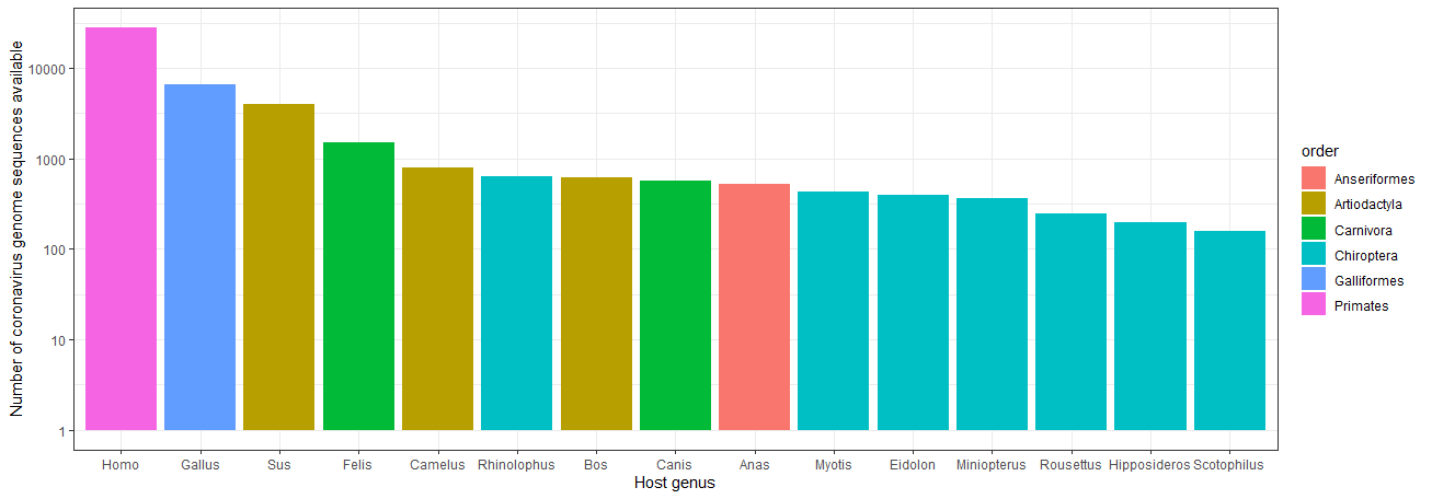
Top fifteen most common animal genera represented in coronavirus genome sequence host metadata, colour-coded by order
While there are a tremendous number of sequences of coronaviruses sampled from humans and domestic animals, there are also quite a few genera of bats present among the most represented hosts! Again, this isn’t particularly surprising, as bats have a rich coevolutionary history with coronaviruses6, which has been an intense focus of study.
🔗 Conclusion
rentrez offers an automated way to search and retrieve genome sequences and metadata, while taxizedb is capable of retrieving and resolving various levels of taxonomic classification. Using these packages in combination represents a reproducible approach to extracting a standardised dataset of coronavirus nucleotide sequences and their sample hosts. This reproducibility is essential for those studies attempting to modelling host-virus relationships to better understand future epidemic threats in humans. I’ve used the above functions to process data to a suitable standard for training machine learning models to predict coronavirus hosts based on their sequence features7. But of course, neither package is limited to viruses; their functionality makes for some brilliant additions to any biologist’s R toolkit!
NCBI GenBank. https://www.ncbi.nlm.nih.gov/genbank/ ↩︎
Winter, D. J. (2017). rentrez: an R package for the NCBI eUtils API. The R Journal, 9(2), 520-526. https://doi.org/10.32614/RJ-2017-058 ↩︎
Liu, P., Jiang, J.Z., Wan, X.F., Hua, Y., Li, L., Zhou, J., Wang, X., Hou, F., Chen, J., Zou, J., & Chen, J. (2020). Are pangolins the intermediate host of the 2019 novel coronavirus (SARS-CoV-2)? PLoS Pathogens, 16(5), e1008421. https://doi.org/10.1371/journal.ppat.1008421 ↩︎
Xiao, K., Zhai, J., Feng, Y., Zhou, N., Zhang, X., Zou, J.J., Li, N., Guo, Y., Li, X., Shen, X., Zhang, Z, Chen, R.A., Wu, Y.J., Peng, S.M., Huang, M., Xie, W.J., Cai, Q.H., Hou, F.H., Chen, W., Xiao, L., & Shen, Y. (2020). Isolation of SARS-CoV-2-related coronavirus from Malayan pangolins. Nature, 583, 286-289. https://doi.org/10.1038/s41586-020-2313-x ↩︎
Chamberlain, S. & Arendsee, Z. (2020). taxizedb: Tools for Working with ‘Taxonomic’ Databases. https://docs.ropensci.org/taxizedb ↩︎
Cui, J., Li, F., & Shi, Z.L. (2019). Origin and evolution of pathogenic coronaviruses. Nature Reviews Microbiology, 17, 181-192. https://doi.org/10.1038/s41579-018-0118-9 ↩︎
Brierley, L., & Fowler, A. (2020). Predicting the animal hosts of coronaviruses from compositional biases of spike protein and whole genome sequences through machine learning. bioRxiv preprint, 2020.11.02.350439. https://doi.org/10.1101/2020.11.02.350439 ↩︎
Filed under
Suggest an edit
Open a pull request
