
Tuesday, December 1, 2020 From rOpenSci (https://ropensci.org/blog/2020/12/01/mcbette-selecting-the-best-inference-model/). Except where otherwise noted, content on this site is licensed under the CC-BY license.
With this blog post, I show how to use the mcbette R package in an informal way. A more formal introduction on mcbette can be found in the Journal of Open Source Science 1. After introducing a concrete problem, I will show how mcbette can be used to solve it.
After discussing mcbette, I will conclude with why I think rOpenSci is important and how enjoyable my experiences have been so far.
🔗 The problem
Imagine you are a field biologist. All around the world, you captured multiple bird species of which you obtained a blood sample. From the blood, you have extracted the DNA. Using DNA, one can determine how these species are evolutionarily related. The problem is, which model of evolution do you assume for your birds?
To illustrate the problem of picking the right model of evolution, we start from the DNA sequences of primates (we will abandon birds here). To be more precise, we will be using a DNA alignment, which are DNA sequences that are arranged in such a way that similar parts of the DNA sequences are at the same position in the sequences. The DNA alignment we use needs first to be converted from NEXUS to FASTA format:
library(beastier) # beastier is part of babette
fasta_filename <- tempfile("primates.fasta")
save_nexus_as_fasta(
  get_beast2_example_filename("Primates.nex"),
  fasta_filename
)
DNA consists of a long string of four different elements called nucleotides, resulting in a four letter alphabet encoding for the proteins a cell needs. In our case, we do not have the full DNA sequence of all primates, but ‘only’ 898 nucleotides. Here I show the DNA sequences:
library(ape)
par0 <- par(mar = c(3, 7, 3, 1))
dna_sequences <- read.FASTA(fasta_filename)
image.DNAbin(dna_sequences, mar = c(3, 7, 3, 1))
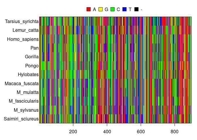
DNA alignment of primates
par(par0)
From this DNA alignment, we can use the R package babette 23 to estimate the evolutionary history of these species.
First, we’ll load babette:
library(babette, quietly = TRUE)
Here, we estimate the evolutionary history of these species:
out <- bbt_run_from_model(fasta_filename)
An evolutionary history can be visualized by a tree-like structure called a phylogeny. babette, however, creates multiple phylogenies of which the more likelier ones show up more often. This results in a visualization that also shows the uncertainty of the inferred phylogenies:
plot_densitree(
  out$primates_trees[9000:10000],
  alpha = 0.01
)
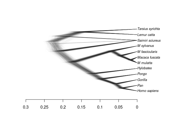
the estimated evolutionary history of primates
🔗 The problem?
As we have observed, inferring the evolutionary history from DNA sequences is easy. The open question is: have we used the best evolutionary model?
This is where mcbette can help out. mcbette is an abbreviation of ‘Model Comparison using babette’ and it helps to pick the best evolutionary model, where ‘best’ is defined as ’the evolutionary model that has been most likely to have generated the alignment, from a set of models’. The addition of ‘from a set of models’ is important, as there are infinitely many evolutionary models to choose from.
So far in this example we have used babette’s default evolutionary model. An evolutionary model consists out of, among others, three most important parts, which are the site, clock and tree model. The site model encompasses the way the (in our case) DNA sequence changes through time. The clock model embodies the rate of change over the different (in our case) species. The tree model specifies the (in our case) speciation model, that is how the branches of the trees are formed.
Let’s figure out what a default babette evolutionary model assumes.
default_model <- create_inference_model()
print(
  paste0(
    "Site model: ", default_model$site_model$name, ". ",
    "Clock model: ", default_model$clock_model$name, ". ",
    "Tree model: ", default_model$tree_prior$name
  )
)
[1] "Site model: JC69. Clock model: strict. Tree model: yule"
Apparently, the default site model embeds a Jukes-Cantor nucleotide substitution model (i.e. all nucleotide mutations are equally likely), the default clock model is strict (i.e. all DNA sequences change at the same rate), and the speciation model is Yule (i.e. speciation rates are constant and extinction rate is zero). These default settings are picked for a reason: these are the simplest site, clock and tree model.
The question is if this default evolutionary model is the most likely to have actually resulted in the original alignment. It is easy to argue that the site, clock and tree model are overly simplistic (they are!).
🔗 The competing model
In this example, I will let the default evolutionary model compete
with only one other evolutionary model.
For this, there are plenty of options! Tip: to get an overview of
all inference models, view the
inference models vignette
of the beautier
package (which is part of babette),
or go to URL https://cran.r-project.org/web/packages/beautier/vignettes/inference_models.html.
Here, I create the competing model:
competing_model <- create_inference_model(
  clock_model = create_rln_clock_model()
)
The competing model has a different clock model: ‘rln’ stands for ‘relaxed log-normal’, which denotes that the different species can have different mutation rates, where these mutation rates follow a log-normal distribution.
🔗 Getting the results
We must modify our inference model first, to prepare them for model comparison:
default_model$mcmc <- create_ns_mcmc(particle_count = 16)
competing_model$mcmc <- create_ns_mcmc(particle_count = 16)
Increasing the number of particles improves the accuracy of the marginal likelihood estimation. Because this accuracy is also estimated, we can also see how strongly to believe a model is better.
Now, we load mcbette, ‘Model Comparison using babette’ to do our model comparison:
library(mcbette)
Then, we let mcbette estimate the marginal likelihoods of both models. The marginal likelihood is the likelihood to observe the data given a model, which is exactly what we need here. Also note that this approach to compare models has no problems to honestly compare models with a different amount of parameters; there is a natural penalty for more models with more parameters.
marg_liks <- est_marg_liks(
  fasta_filename = fasta_filename,
  inference_models = list(
    default_model,
    competing_model
  )
)
Note that this calculation takes quite some time!
Here we show the results as table:
knitr::kable(marg_liks)
| site_model_name | clock_model_name | tree_prior_name | marg_log_lik | marg_log_lik_sd | weight | ess |
|---|---|---|---|---|---|---|
| JC69 | strict | yule | -6481.435 | 1.794633 | 0.0457542 | 146.7444 |
| JC69 | relaxed_log_normal | yule | -6478.397 | 1.792379 | 0.9542458 | 220.6656 |
The most important column to look at here is the weight column.
All (two) weights sum up to one. A model’s weight is its relative
chance to have observed the alignment given the model. As can
be seen, the weight for the more complex (relaxed log-normal)
clock model is higher (i.e. 0.9343919).
We can also visualize which model is the best, by plotting the estimated marginal likelihoods and the error in this estimation:
plot_marg_liks(marg_liks)
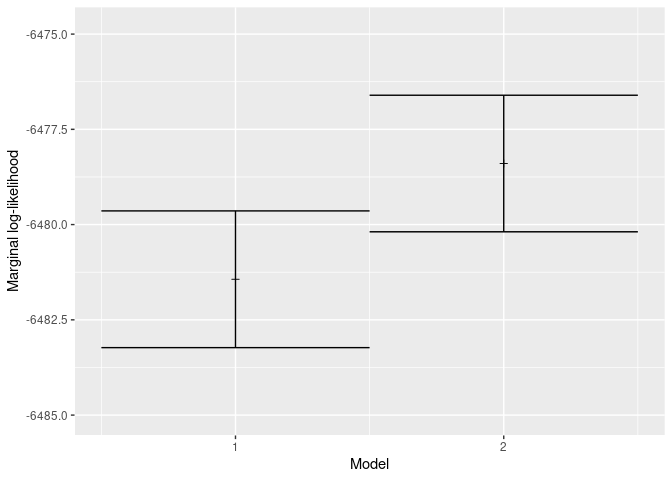
the estimated marginal likelihoods
Note that marginal likelihoods can be very close to zero. Hence, mcbette use log values. The model with the lowest log value, thus has the highest marginal likelihood and is thus more likely to have resulted in the data.
🔗 Why rOpenSci?
I enjoy rOpenSci, because I care about my users: rOpenSci allows me to prove that I do so.
I feel it is a misconception that free software is always beneficial.
I would claim that free software is beneficial only, when its developers
observably care about their users. For starters, there should be a place
to submit bug reports (e.g. GitHub), instead of using a package-related
email address (e.g. [email protected]) that gets
forgotten by the developer. A user needs a place to ask questions and
submit bug reports. A young researcher may base their next research
on a newly developed package, only to result in weeks of frustration
due to the package maintainer’s inconsideration.
I feel it makes the world a better place,
that rOpenSci requires its developers to use a website to submit bug reports.
To ensure that I am considerate towards my users, rOpenSci provides me with my first critical test users of my packages. I know what I expect my package to do, yet cannot predict well what others think. Also, although I attempt to write exemplary code (and documentation, tests, etc.), I will forget some little things in the process. During the rOpenSci review, my reviewers (Joëlle Barido-Sottani, David Winter and Vikram Baliga) have impressed me by pointing out each of these (many!) little details I missed and it has taken me weeks to process all the feedback. My rOpenSci reviewers have made my code better in ways I did not imagine.
Whenever I can, I use packages reviewed by rOpenSci: it is where the awesome and considerate people are!
🔗 References
Bilderbeek (2020) mcbette: model comparison using babette. Journal of Open Source Software, 5(54), 2762. https://doi.org/10.21105/joss.02762 ↩︎
Bilderbeek and Etienne (2018) babette: BEAUti 2, BEAST2 and Tracer for R. Methods in Ecology and Evolution 9, no. 9: 2034-2040. https://doi.org/10.1111/2041-210X.13032 ↩︎
Bilderbeek (2020) Call BEAST2 for Bayesian evolutionary analysis from R. rOpenSci blog post. https://ropensci.org/blog/2020/01/28/babette/ ↩︎
Filed under
Suggest an edit
Open a pull request
