
Tuesday, June 8, 2021 From rOpenSci (https://ropensci.org/blog/2021/06/08/world-ocean-day/). Except where otherwise noted, content on this site is licensed under the CC-BY license.
Happy World Ocean Day!
World Ocean Day is a day of celebration and action to protect our shared ocean.
While I already appreciate the importance of protecting sensitive ecosystems, including the ocean1, I found the idea of World Ocean Day especially touching.
On World Ocean Day, people around our blue planet celebrate and honor our one shared ocean, that connects us all.
This year has been hard, and like many, I often feel isolated and emotionally exhausted. The idea that we have only one ocean and it connects us is a lovely way to remember that as isolated as we may feel we’re all here on this planet together.
So in honour of World Ocean Day, let’s take a look at some important ocean metrics using open data and open software via rOpenSci packages!
🔗 Sea ice
One of the biggest challenges for protecting our ocean is climate change2. Last September the Arctic sea ice had the 2nd-lowest extent in a 40-year record3. This isn’t good for the Arctic ecosystem and has impacts not only on wildlife but on humans as well 4. 😿
Let’s see if we can’t explore ice extent ourselves using open data and open source packages that are part of the rOpenSci package collections.
Here, we’ll use two rOpenSci packages
- rnoaa to access NOAA data on sea ice coverage5
- and rnaturalearth to get coastal outlines for context
Both these packages can do so much more, so check out the docs if you’re curious. rnoaa is by Scott Chamberlain for rOpenSci and rnaturalearth is by Andy South, peer reviewed through rOpenSci.
We’ll also use sf for working with spatial data, dplyr for data manipulation, and ggplot2 for plotting.
library(rnoaa)
library(rnaturalearth)

library(sf)
library(ggplot2)
library(dplyr)
Let’s get some ice data!
We’ll use the sea_ice() function to grab data on ice extent for every 5 years from 1980 to 2020 (year = seq(1980, 2020, 5)), in September (month = "Sep"), and for the Arctic (North) (pole = "N").
ice <- sea_ice(year = seq(1980, 2020, 5), month = "Sep", pole = "N")
ice is a list, with each list item corresponding to a year.
Let’s take a brief look at what we’ve got, by scanning the head() of the first two years worth of data.
head(ice[[1]])
     long     lat order  hole piece id group
1  125000 2100000     1 FALSE     1  0   0.1
2  150000 2100000     2 FALSE     1  0   0.1
3  150000 2075000     3 FALSE     1  0   0.1
4  125000 2075000     4 FALSE     1  0   0.1
5  125000 2100000     5 FALSE     1  0   0.1
6 -175000 2025000     1 FALSE     1  1   1.1
head(ice[[2]])
     long     lat order  hole piece id group
1  125000 2100000     1 FALSE     1  0   0.1
2  150000 2100000     2 FALSE     1  0   0.1
3  150000 2075000     3 FALSE     1  0   0.1
4  125000 2075000     4 FALSE     1  0   0.1
5  125000 2100000     5 FALSE     1  0   0.1
6 -175000 2025000     1 FALSE     1  1   1.1
Each year is a ‘fortified’ data frame which you could plot using geom_polygon().
But I want to get the projection right, so let’s bind the rows together (adding year as a parameter) and convert to an sf object.
We’ll transform to EPSG 3411 which refers to the NSIDC Sea Ice Polar Stereographic North projection commonly used to map the Arctic.
ice_sf <- ice %>%
  bind_rows(.id = "year") %>%
  mutate(year = factor(year, labels = seq(1980, 2020, 5))) %>%
  st_as_sf(coords = c("long", "lat"), crs = 3411)
ice_sf
Simple feature collection with 13639 features and 6 fields
Geometry type: POINT
Dimension:     XY
Bounding box:  xmin: -2550000 ymin: -3250000 xmax: 2350000 ymax: 4950000
Projected CRS: NSIDC Sea Ice Polar Stereographic North
First 10 features:
   year order  hole piece id group                geometry
1  1980     1 FALSE     1  0   0.1  POINT (125000 2100000)
2  1980     2 FALSE     1  0   0.1  POINT (150000 2100000)
3  1980     3 FALSE     1  0   0.1  POINT (150000 2075000)
4  1980     4 FALSE     1  0   0.1  POINT (125000 2075000)
5  1980     5 FALSE     1  0   0.1  POINT (125000 2100000)
6  1980     1 FALSE     1  1   1.1 POINT (-175000 2025000)
7  1980     2 FALSE     1  1   1.1 POINT (-150000 2025000)
8  1980     3 FALSE     1  1   1.1   POINT (-150000 2e+06)
9  1980     4 FALSE     1  1   1.1   POINT (-175000 2e+06)
10 1980     5 FALSE     1  1   1.1 POINT (-175000 2025000)
This results in a collection of points, so we’ll want to summarize() the data into multipoints by year and group, and then st_cast() into polygons.
ice_sf <- ice_sf %>%
  group_by(year, group) %>%
  summarize(do_union = FALSE, .groups = "drop") %>%
  st_cast(to = "POLYGON")
ice_sf
Simple feature collection with 1013 features and 2 fields
Geometry type: POLYGON
Dimension:     XY
Bounding box:  xmin: -2550000 ymin: -3250000 xmax: 2350000 ymax: 4950000
Projected CRS: NSIDC Sea Ice Polar Stereographic North
# A tibble: 1,013 x 3
   year  group                                                          geometry
   <fct> <fct>                                                     <POLYGON [m]>
 1 1980  0.1   ((125000 2100000, 150000 2100000, 150000 2075000, 125000 2075000…
 2 1980  1.1   ((-175000 2025000, -150000 2025000, -150000 2e+06, -175000 2e+06…
 3 1980  2.1   ((-1350000 1900000, -1250000 1900000, -1250000 1875000, -1275000…
 4 1980  3.1   ((-1250000 1875000, -1225000 1875000, -1225000 1850000, -1250000…
 5 1980  4.1   ((-1200000 1875000, -1175000 1875000, -1175000 1850000, -1200000…
 6 1980  5.1   ((425000 1800000, 450000 1800000, 450000 1775000, 425000 1775000…
 7 1980  6.1   ((-350000 1675000, -325000 1675000, -325000 1650000, -350000 165…
 8 1980  7.1   ((-2e+06 1650000, -1975000 1650000, -1975000 1600000, -2e+06 160…
 9 1980  8.1   ((750000 1625000, 875000 1625000, 875000 1600000, 850000 1600000…
10 1980  9.1   ((-2075000 1525000, -2050000 1525000, -2050000 1500000, -2075000…
# … with 1,003 more rows
Here it’s important to use do_union = FALSE because we don’t want the order of the points to change (otherwise when we plot we’ll get @accidental__aRt!)
Let’s take a peak at what we’ve got
ggplot() +
  theme_minimal() +
  geom_sf(data = ice_sf, aes(fill = year), colour = NA)
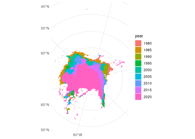
Oooo very nice! But a couple of points could be improved
- It’s a bit hard to understand the context because there’s no land
- Some points up around ~45 degrees North look highly improbable for sea ice
- I think we can do better than ggplot2 default colours 😁
First we’ll crop out that questionable data.
We can see the extent of the data with st_bbox().
st_bbox(ice_sf)
    xmin     ymin     xmax     ymax
-2550000 -3250000  2350000  4950000
It seems like that high ymax value is probably the culprit.
In the figure above, the y extents (circular axes) look roughly symmetrical.
So, let’s do a rough crop and see where it gets us.
Note that I’m also using st_make_valid() to fix a bit of ring self-intersection that pops up as an error otherwise.
ice_sf <- ice_sf %>%
  st_make_valid() %>%
  st_crop(xmin = -2550000, ymin = -3250000, xmax = 2350000, ymax = 3500000)
Warning: attribute variables are assumed to be spatially constant throughout all
geometries
ggplot() +
  theme_minimal() +
  geom_sf(data = ice_sf, aes(fill = year), colour = NA)
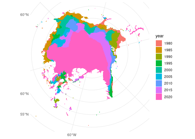
Much better! There are definitely more precise and sophisticated ways of filtering or cropping spatial data, but this will do for now.
Next, let’s get the coastline spatial data using rnaturalearth’s function ne_coastlines().
We’ll get medium quality, return it as sf, then transform and crop to match the projection and extent of our ice data.
coast <- ne_coastline(scale = "medium", returnclass = "sf") %>%
  st_transform(crs = st_crs(ice_sf)) %>%
  st_crop(st_bbox(ice_sf))
Warning: attribute variables are assumed to be spatially constant throughout all
geometries
Now let’s take another stab at mapping, using the coastline data as well as viridis scales.
ggplot() +
  theme_minimal() +
  geom_sf(data = ice_sf, aes(fill = year), colour = NA) +
  geom_sf(data = coast) +
  scale_fill_viridis_d(option = "inferno", begin = 0.1, end = 0.9)
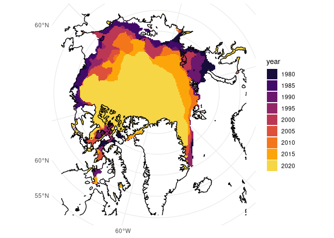
From here, it’s very apparent how much the ice extent in September has changed over the years. There’s been a fair amount of reduction especially along Russia’s (top and top right) and Alaska’s (left) coasts, and among Canada’s Arctic Archipelago (bottom left).
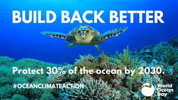
This isn’t great news, and it’s not new news, but as World Ocean Day is about calls to action, specifically for protecting 30% of the planet’s land and ocean by 2030, it’s always worth the reminder that conservation is important.
🔗 Leopard seals
One of my favourite videos is a TED Talk by Paul Nicklen: Animal tales from icy wonderlands. It’s a fantastic view of life in the polar oceans and an amazing story of a photographer and a leopard seal.
So in honour of that wonderful story, let’s do another exploration of the ocean, but this time by looking at leopard seals in Antarctica!
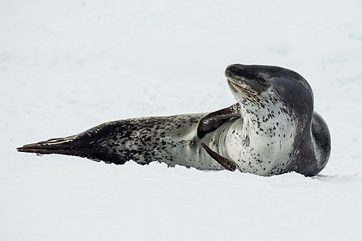
Andrew Shiva / Wikipedia / CC BY-SA 4.0
In addition to rnaturalearth, sf, dplyr, and ggplot2 which we loaded above, we’ll use lubridate to handle date/times, and the rOpenSci package rinat, for accessing species observations from the citizen science project iNaturalist. rinat is by Ted Hart and Stéphane Guillou.
library(rinat)
library(lubridate)
We’ll use get_inat_obs() from rinat, then will select() columns for dates, descriptions and coordinates.
We’ll filter() out records without a date and those farther away from Antarctica, convert to proper dates, and extract the year().
seals <- get_inat_obs(taxon_name = "leopard seal") %>%
  select(scientific_name, datetime, description, latitude, longitude) %>%
  filter(datetime != "") %>%
  mutate(datetime = ymd_hms(datetime),
         year = year(datetime))
glimpse(seals)
Rows: 99
Columns: 6
$ scientific_name <chr> "Hydrurga leptonyx", "Hydrurga leptonyx", "Hydrurga le…
$ datetime        <dttm> 2021-05-25 00:09:12, 2021-05-07 01:56:37, 2020-01-12 …
$ description     <chr> "Identified as Owha. Unfortunately she was scared off …
$ latitude        <dbl> -36.87974, -36.77027, -63.39282, -64.15940, -63.19452,…
$ longitude       <dbl> 174.66350, 174.66345, -54.59607, -60.92037, -57.31312,…
$ year            <dbl> 2021, 2021, 2020, 2020, 2020, 2019, 2018, 2019, 2012, …
Alright, we have 59 observations of leopard seals around Antarctica, let’s see where they’re from.
As before, we’ll turn this into spatial data by using the longitude and latitude columns as our coordinates.
Because we’re dealing with Lon/Lat (GPS data), we’ll specify the starting crs as EPSG 4326, which refers to the World Geodetic System (WGS84).
We’ll end by transforming to a projection more appropriate for the Antarctic, EPSG 3412.
seals_sf <- seals  %>%
  st_as_sf(coords = c("longitude", "latitude"), crs = 4326) %>%
  st_transform(3412)
Let’s get a land mass to plot our points on, for context.
antarctic <- ne_countries(returnclass = "sf") %>%
  st_transform(3412) %>%     # CRS for the Antarctic
  st_make_valid() %>%        # To avoid intersection errors
  st_crop(st_bbox(seals_sf)) # Crop to our data
Warning: attribute variables are assumed to be spatially constant throughout all
geometries
Finally, let’s take a look!
ggplot() +
  geom_sf(data = antarctic, fill = "grey") +
  geom_sf(data = seals_sf, aes(colour = year)) +
  scale_colour_viridis_c(end = 0.85)
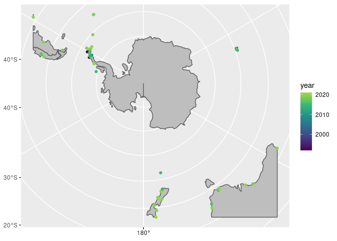
Looks like most observations are around the Antarctic Peninsula, let’s take a closer look!
(Here I got the starting limits from the information in seals_sf and then just trial-and-errored until I got the window I wanted).
ggplot() +
  geom_sf(data = antarctic, fill = "grey") +
  geom_sf(data = seals_sf, aes(colour = year)) +
  scale_colour_viridis_c(end = 0.85) +
  coord_sf(xlim = c(-3099695, -1500000), ylim = c(400000, 3190715))
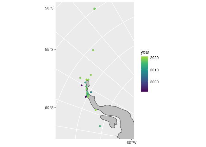
There you have it, all the leopard seal observations around the Antarctic Peninsula by year. I wonder if this is because there are so many research stations in the area?
And let’s not forget to enjoy some of the descriptions:
filter(seals, description != "") %>%
  slice(1:7) %>%
  pull(description)
[1] "Identified as Owha. Unfortunately she was scared off by a fisherman with a piper net. "
[2] "a marine mammal found at people's private dock around Herald Island"
[3] "eating an adelie penguin"
[4] "Eating a Gentoo penguin"
[5] "Eating Gentoo penguins"
[6] "Resting on the beach."
[7] "The seal raised its head every time a vehicle passed on the road behind the beach.\n\nApparently it had been seen on various beaches in the area for the week preceding this observation."
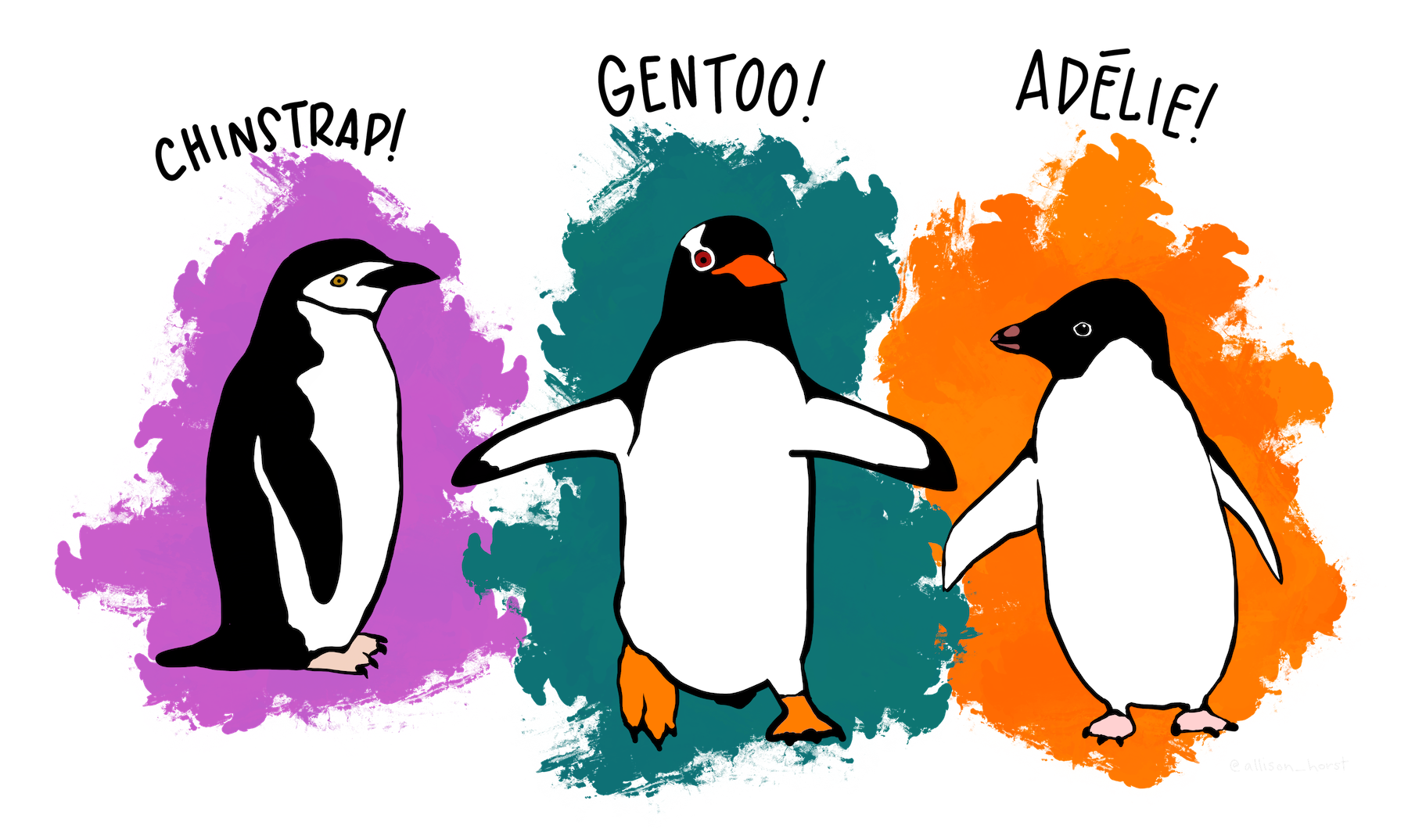
Artwork by Allison Horst
🔗 Learn more about these awesome packages
- 2018-12-04 rOpenSci blog “rnoaa: new data sources and NCDC units” by Scott Chamberlain
- 2014-03-13 rOpenSci blog “rnoaa - Access to NOAA National Climatic Data Center data” by Scott Chamberlain
- Use cases
🔗 Other rOpenSci resources for studying the ocean:
- 2019-11-13 rOpenSci blog “The Antarctic/Southern Ocean rOpenSci community”
- by Ben Raymond and Michael Sumner (with examples)
- antanym by Ben Raymond
- Tools and info on Antarctic geographic place names
- dataaimsr by Diego Barneche
- Access data from Australian Institute of Marine Science (AIMS)
- mregions by Scott Chamberlain and Lennert Schepers
- Access Marine Regions info
- ramlegacy by Kshitiz Gupta
- Access RAM legacy Stock Assessment Data Base (compilation of stock assessment results for commercially exploited marine populations)
- rfishbase by Carl Boettiger
- Access FishBase information on most known species of fish
- wateRinfo by Stijn Van Hoey - Access water and weather info for Flanders, Belgium
- worrms by Scott Chamberlain for rOpenSci
- Access the World Register of Marine Species (WoRMS)
🔗 Have you used rOpenSci packages to study our ocean?
We’d love to share your examples! Consider adding your use cases (description and code snippet or link to code/post) to the rOpenSci public forum.
There’s a template to help & we’ll tweet any posted to share uses of rOpenSci packages.
Take care and remember to celebrate World Ocean Day!
Why should we care about the ocean https://oceanservice.noaa.gov/facts/why-care-about-ocean.html ↩︎
The Ocean and Climate Change https://www.iucn.org/resources/issues-briefs/ocean-and-climate-change ↩︎
Arctic Report Card: Update for 2020 https://arctic.noaa.gov/Report-Card/Report-Card-2020/ArtMID/7975/ArticleID/891/Sea-Ice ↩︎
Six ways loss of Arctic ice impacts everyone https://www.worldwildlife.org/pages/six-ways-loss-of-arctic-ice-impacts-everyone; Climate Change In The Arctic: An Inuit Reality https://www.un.org/en/chronicle/article/climate-change-arctic-inuit-reality ↩︎
There’s also the new seaice package by the Australian Antarctic Division https://github.com/AustralianAntarcticDivision/seaice ↩︎
Filed under
Suggest an edit
Open a pull request

_04.jpg)