
Tuesday, July 26, 2022 From rOpenSci (https://ropensci.org/blog/2022/07/26/package-yfr/). Except where otherwise noted, content on this site is licensed under the CC-BY license.
Package yfR recently passed peer review at rOpenSci and is all about downloading stock price data from Yahoo Finance (YF). I wrote this package to solve a particular problem I had as a teacher: I needed a large volume of clean stock price data to use in my classes, either for explaining how financial markets work or for class exercises. While there are several R packages to import raw data from YF, none solved my problem.
Package yfR facilitates the importation of data, organizing it in the tidy format and speeding up the process using a cache system and parallel computing. yfR is a backwards-incompatible substitute of BatchGetSymbols, released in 2016 (see vignette yfR and BatchGetSymbols for details).
Introducing yfR
Yahoo Finance provides a vast repository of stock price data around the globe. It covers a significant number of markets and assets, and is therefore used extensively in academic research and teaching. In order to import the financial data from YF, all you need is a ticker (id of a stock, e.g. “GM” for General Motors) and a time period – first and last date.
🔗 Features of yfR
Package yfR distinguishes itself from other similar packages with the following features:
Fetches daily/weekly/monthly/annual stock prices/returns from yahoo finance and outputs a dataframe (tibble) in the long format (stacked data);
A feature called collections facilitates download of multiple tickers from a particular market/index. You can, for example, download data for all stocks in the SP500 index with a simple call to
yf_collection_get("SP500");A session-persistent smart cache system is available by default. This means that the data is saved locally and only missing portions are downloaded, if needed.
All dates are compared to a benchmark index such as SP500 (^GSPC) and, whenever an individual asset does not have a sufficient number of dates, the software drops it from the output. This means you can choose to ignore tickers with a high proportion of missing dates.
A customized function called
yf_convert_to_wide()can transform the long dataframe into a wide format (tickers as columns), which is much used in portfolio optimization. The output is a list where each element is a different target variable (prices, returns, volumes).Parallel computing with package furrr is available, speeding up the data importation process.
🔗 Available columns
The main function of the package, yfR::yf_get, returns a dataframe with the financial data. All price data is measured at the unit of the financial exchange. For example, price data for GM (NASDAQ/US) is measured in US dollars, while price data for PETR3.SA (B3/BR) is measured in Reais (Brazilian currency).
The returned data contains the following columns:
ticker: The requested tickers (ids of stocks);
ref_date: The reference day (this can also be year/month/week when using argument freq_data);
price_open: The opening price of the day/period;
price_high: The highest price of the day/period;
price_close: The closing/last price of the day/period;
volume: The financial volume of the day/period, in the unit of the exchange;
price_adjusted: The stock price adjusted for corporate events such as
splits, dividends and others – this is usually what you want/need for studying
stocks as it represents the real financial performance of stockholders;
ret_adjusted_prices: The arithmetic or log return (see input type_return) for the adjusted stock
prices;
ret_adjusted_prices: The arithmetic or log return (see input type_return) for the closing stock
prices;
cumret_adjusted_prices: The accumulated arithmetic/log return for the period (starts at 100%).
Installation
Package yfR is available in its stable version in CRAN, but you can also find the latest features and bug fixes in GitHub and rOpenSci repository. Below you can find the R commands for installation in each case.
# CRAN (stable)
install.packages('yfR')

# GitHub (dev version)
devtools::install_github('ropensci/yfR')

# rOpenSci
install.packages("yfR", repos = c("https://ropensci.r-universe.dev", "https://cloud.r-project.org"))
Examples of usage
🔗 The SP500 historical performance
In this example we are going to download price data for the SP500 index from 1950 to today (2022-07-25), analyze its financial performance and also visualize its prices using ggplot2.
library(yfR)
library(lubridate) # for date manipulations
library(dplyr) # for data manipulations

# set options for algorithm
my_ticker <- '^GSPC'
first_date <- "1950-01-01"
last_date <- Sys.Date()

# fetch data
df_yf <- yf_get(tickers = my_ticker,
                first_date = first_date,
                last_date = last_date)

# output is a tibble with data
glimpse(df_yf)
Rows: 18,257
Columns: 11
$ ticker                 <chr> "^GSPC", "^GSPC", "^GSPC", "^GSPC", "^GSPC", "^…
$ ref_date               <date> 1950-01-03, 1950-01-04, 1950-01-05, 1950-01-06…
$ price_open             <dbl> 16.66, 16.85, 16.93, 16.98, 17.08, 17.03, 17.09…
$ price_high             <dbl> 16.66, 16.85, 16.93, 16.98, 17.08, 17.03, 17.09…
$ price_low              <dbl> 16.66, 16.85, 16.93, 16.98, 17.08, 17.03, 17.09…
$ price_close            <dbl> 16.66, 16.85, 16.93, 16.98, 17.08, 17.03, 17.09…
$ volume                 <dbl> 1260000, 1890000, 2550000, 2010000, 2520000, 21…
$ price_adjusted         <dbl> 16.66, 16.85, 16.93, 16.98, 17.08, 17.03, 17.09…
$ ret_adjusted_prices    <dbl> NA, 0.0114045618, 0.0047477745, 0.0029533373, 0…
$ ret_closing_prices     <dbl> NA, 0.0114045618, 0.0047477745, 0.0029533373, 0…
$ cumret_adjusted_prices <dbl> 1.000000, 1.011405, 1.016206, 1.019208, 1.02521…
The output of yfR is a tibble (dataframe) with the stock price data. We can use it to 1) get the number of years within the data, and 2) calculate the annual financial performance of the index:
n_years <- interval(min(df_yf$ref_date),
                    max(df_yf$ref_date))/years(1)

total_return <- last(df_yf$price_adjusted)/first(df_yf$price_adjusted) - 1

cat(paste0("n_years = ", n_years, "\n",
           "total_return = ",total_return))
n_years = 72.5479452054795
total_return = 236.792910144058
In 1950-01-03, the index was valued at 16.66. Today (2022-07-25), after roughly 72 years, the value of the index is 3961.629883. The total return for the SP500, without accounting for inflation, is equivalent to an impressive 23 679%! Overall, anyone holding stocks for that long has done very well financially.
Additionally, we can also calculate performance as the compounded annual return, which is the usual figure reported when looking stocks in the long run:
ret_comp <- (1 + total_return)^(1/n_years)  - 1

cat(paste0("Comp Return = ",
           scales::percent(ret_comp, accuracy = 0.01)))
Comp Return = 7.83%
Over the 72 of existence, the SP500 index returned an annual compounded interest of 7.83%. This is quite in line with the roughly 8% per year reported in the media.
To visualize the data, we can use a log plot and see the value of the SP500 index over time:
library(ggplot2)

p <- ggplot(df_yf, aes(x = ref_date, y = price_adjusted)) +
  geom_line() +
  labs(
    title = paste0("SP500 Index Value (",
                   year(min(df_yf$ref_date)), ' - ',
                   year(max(df_yf$ref_date)), ")"
    ),
    x = "Time",
    y = "Index Value",
    caption = "Data from Yahoo Finance <https://finance.yahoo.com/>") +
  theme_light() +
  scale_y_log10()

p
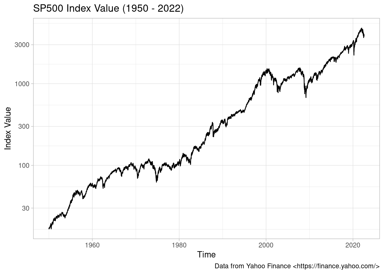
SP500 index value since 1950
🔗 Performance of many stocks
In this second example, instead of using a single stock/index, we will investigate the financial performance of a set of ten stocks using dplyr. First, let’s download the current composition of the SP500 index and select 10 random stocks.
set.seed(20220713)

n_tickers <- 10
df_sp500 <- yf_index_composition("SP500")
✔ Got SP500 composition with 503 rows
rnd_tickers <- sample(df_sp500$ticker, n_tickers)

cat(paste0("The selected tickers are: ",
           paste0(rnd_tickers, collapse = ", ")))
The selected tickers are: AAPL, DHI, AMZN, CMS, FCX, NRG, EXR, CFG, CI, AWK
And now we fetch the data using yfR::yf_get:
df_yf <- yf_get(tickers = rnd_tickers,
                first_date = '2010-01-01',
                last_date = Sys.Date())
Out of the 10 stocks, one was left out due to the high number of missing days. Internally, yf_get compares every ticker to a benchmark time series, in this case the SP500 index itself (see yf_get’s argument bench_ticker). Whenever the proportion of missing days is higher than the default case (thresh_bad_data = 0.75), the algorithm drops the ticker from the output. In the end, we are left with just nine stocks.
First, let’s look at their accumulated return over time:
library(ggplot2)

p <- ggplot(df_yf,
            aes(x = ref_date,
                y = cumret_adjusted_prices,
                color = ticker)) +
  geom_line() +
  labs(
    title = paste0("SP500 Index Value (",
                   year(min(df_yf$ref_date)), ' - ',
                   year(max(df_yf$ref_date)), ")"
    ),
    x = "Time",
    y = "Accumulated Return (from 100%)",
    caption = "Data from Yahoo Finance <https://finance.yahoo.com/>") +
  theme_light() +
  scale_y_log10()

p
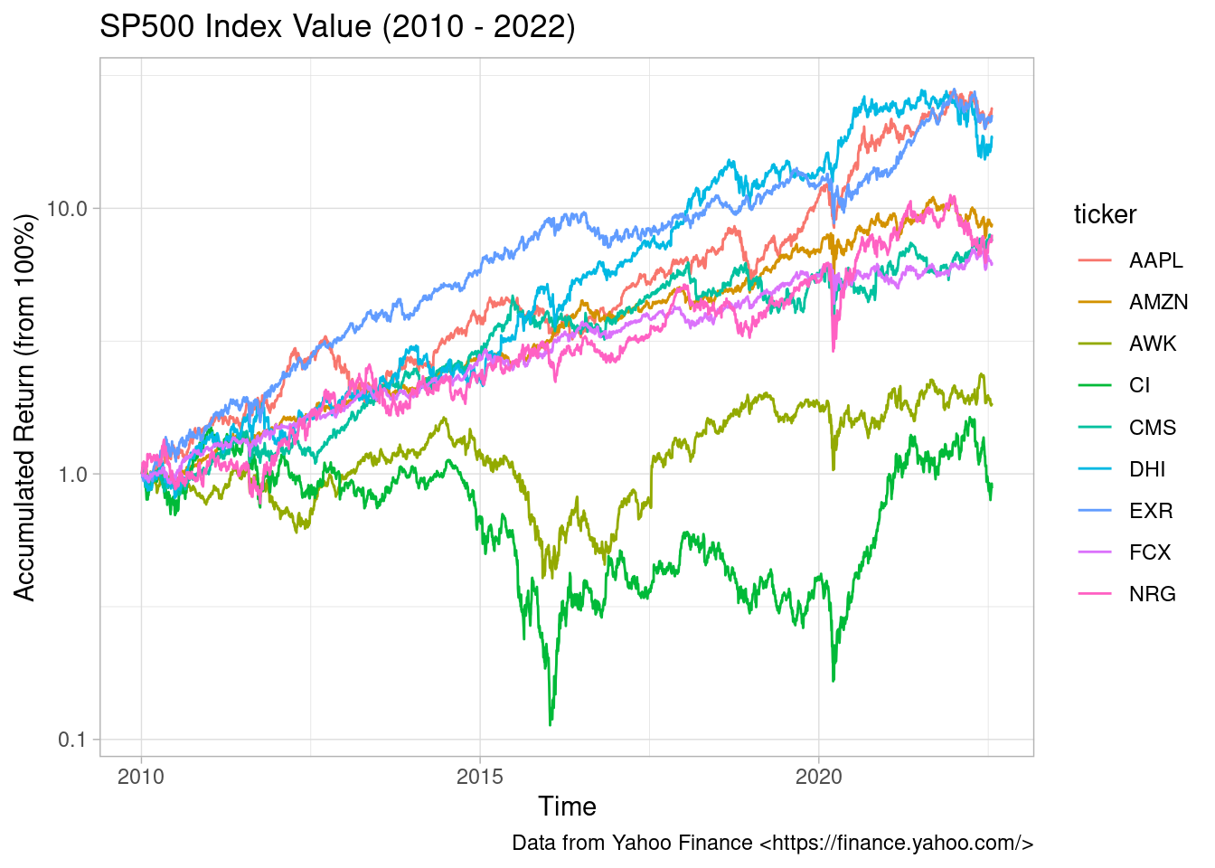
Accumulated Return of 9 stocks
As we can see, some stocks, such as AMZN and AAPL, did much better than others. We can check this numerically by reporting their compounded return over the period:
library(dplyr)

tab_perf <- df_yf |>
  group_by(ticker) |>
  summarise(
    n_years = interval(min(ref_date),
                       max(ref_date))/years(1),
    total_ret = last(price_adjusted)/first(price_adjusted) - 1,
    ret_comp = (1 + total_ret)^(1/n_years) - 1
  )

tab_perf |>
  mutate(n_years = floor(n_years),
         total_ret = scales::percent(total_ret),
         ret_comp = scales::percent(ret_comp)) |>
  knitr::kable(caption = "Financial Performance of Several Stocks")
Table: Table 1: Financial Performance of Several Stocks
| ticker | n_years | total_ret | ret_comp |
|---|---|---|---|
| AAPL | 12 | 2 258% | 28.65% |
| AMZN | 12 | 1 729% | 26.07% |
| AWK | 12 | 776% | 18.88% |
| CI | 12 | 665% | 17.61% |
| CMS | 12 | 526% | 15.74% |
| DHI | 12 | 696% | 17.98% |
| EXR | 12 | 2 146% | 28.15% |
| FCX | 12 | -12% | -0.99% |
| NRG | 12 | 81% | 4.85% |
Final thoughts
Package yfR was created to facilitate the importation and organization of YF data sets. In the examples of this post, we can see how easy it is to download the data and do some simple performance statistics. We only scratched the surface, there are many ways to analyze stock data, not just financial performance.
Acknowledgements
Package yfR was reviewed by Alexander Fischer and Nic Crane, and I’m very grateful for their feedback, which improved the package significantly. I’m also grateful to Joshua Ulrich, the maintainer of quantmod, which wrote quantmod::getSymbols, the main function used by yfR::yf_get
Filed under
Suggest an edit
Open a pull request
