Introducing distionary for Building and Probing Distributions

After passing through rOpenSci peer review, the distionary package is now newly available on CRAN. It allows you to make probability distributions quickly – either from a few inputs or from its built-in library – and then probe them in detail.

These distributions form the building blocks that piece together advanced statistical models with the wider probaverse ecosystem, which is built to release modelers from low-level coding so production pipelines stay human-friendly. Right now, the other probaverse packages are distplyr, allowing you to morph distributions into new forms, and famish, allowing you to tune distributions to data. Developed with risk analysis use cases like climate and insurance in mind, the same tools translate smoothly to simulations, teaching, and other applied settings.

This post highlights the top 3 features of this youngest version of distionary. Let’s start by loading the package.

library(distionary)

🔗 Feature 1: more than just Base R distributions

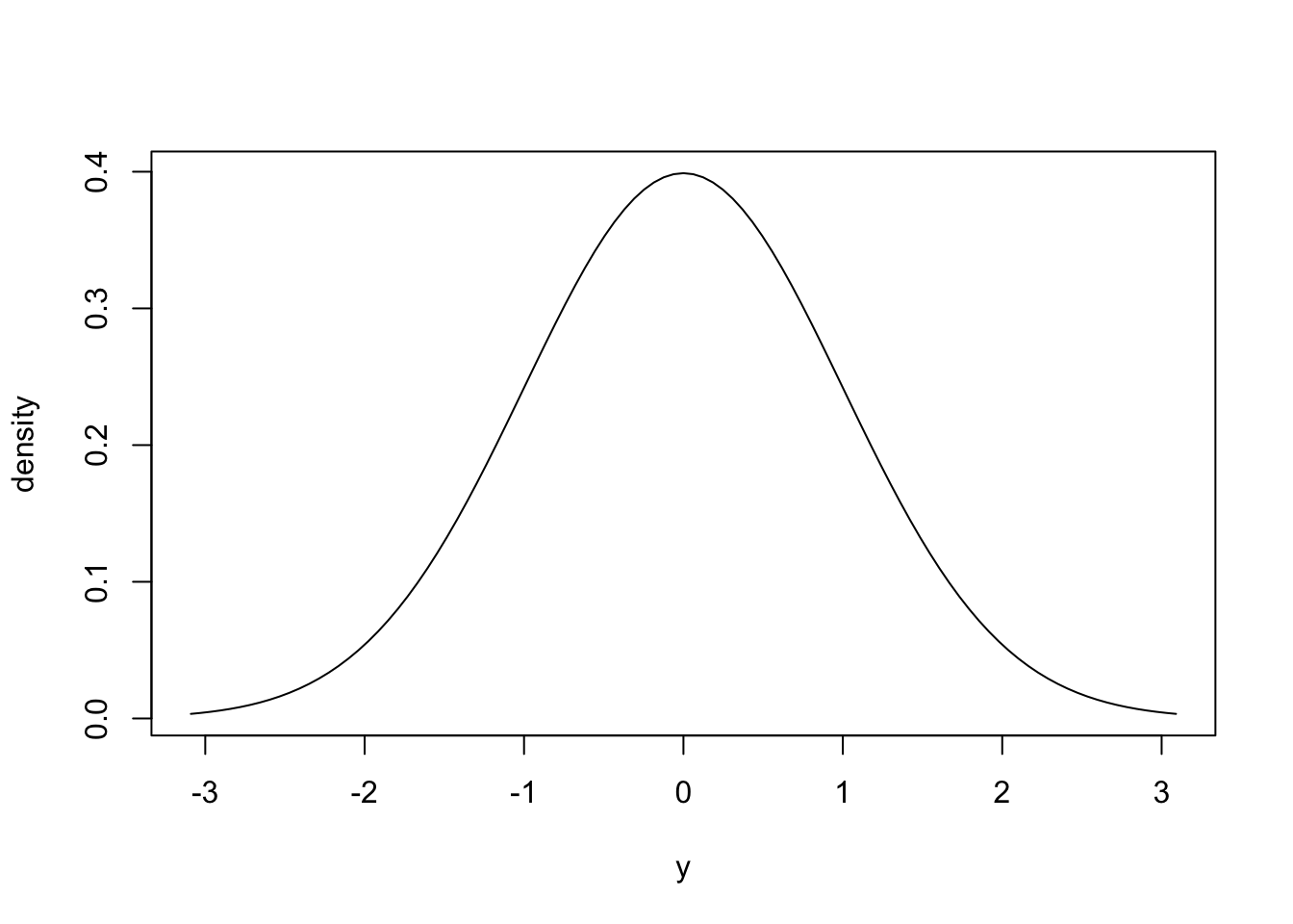
Of course, all the Base R distributions are available in distionary. Here’s everyone’s favourite Normal distribution.

dst_norm(0, 1)

Normal distribution (continuous) 
--Parameters--
mean   sd 
   0    1 

plot(dst_norm(0, 1))

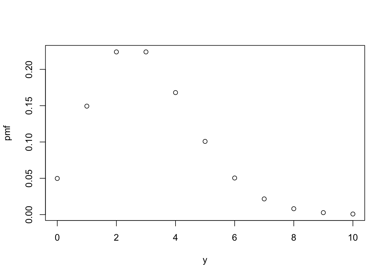
And good old Poisson.

dst_pois(3)

Poisson distribution (discrete) 
--Parameters--
lambda 
     3 

plot(dst_pois(3))

But there are additional game-changing distributions included, too.

A Null distribution, which always evaluates to NA. When you’re running an algorithm that encounters an issue, you can return a Null distribution instead of throwing an error. Even downstream evaluation steps won’t error out because the code still sees a distribution rather than a bare NA or NULL.

# Make a Null distribution.
null <- dst_null()
# Null distributions always evaluate to NA.
eval_quantile(null, at = c(0.25, 0.5, 0.75))

[1] NA NA NA

mean(null)

[1] NA

Empirical distributions, where the data are the distribution. These respect observed behaviour without forcing a specific shape, and are also commonly used as a benchmark for comparison against other models. Here’s an example using the Ozone concentration from the airquality dataset that comes loaded with R.

# Empirical distribution of Ozone from the `airquality` dataset.
emp <- dst_empirical(airquality$Ozone, na_action_y = "drop")
# Inspect
print(emp, n = 5)

Finite distribution (discrete) 
--Parameters--
# A tibble: 67 × 2
  outcomes   probs
     <int>   <dbl>
1        1 0.00862
2        4 0.00862
3        6 0.00862
4        7 0.0259 
5        8 0.00862
# ℹ 62 more rows

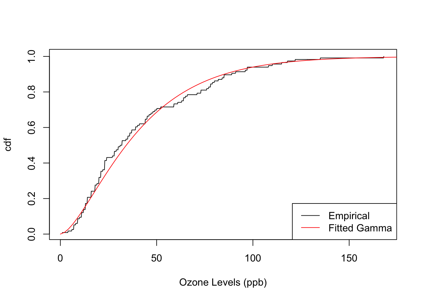
Compare its cumulative distribution function (CDF) to that of a Gamma distribution fitted to the Ozone levels, borrowing the probaverse’s famish package for the fitting task.

# Fit a Gamma distribution to Ozone using the famish package.
library(famish)
gamma <- fit_dst_gamma(airquality$Ozone, na_action = "drop")

# Plot the cumulative distribution functions (CDFs) together.
plot(emp, "cdf", n = 1000, xlab = "Ozone Levels (ppb)")
plot(gamma, "cdf", add = TRUE, col = "red")
legend(
  "bottomright",
  legend = c("Empirical", "Fitted Gamma"),
  col = c("black", "red"),
  lty = 1
)

These textbook distributions become much more useful once they become building blocks for building up a system. For example, they could form predictive distributions in a machine learning context, or be related to other variables. This is what the probaverse seeks to make possible.

🔗 Feature 2: friendly towards tidy tabular workflows

First, load the tidyverse to activate tidy tabular workflows. And yes, probaverse is named after the tidyverse because it aims to be a “tidyverse for probability”.

library(tidyverse)

You can safely ignore this next chunk unless you want to see how I’m wrangling some financial data for you.

# Wrangle the stocks data frame using tidyverse.
stocks <- as_tibble(EuStockMarkets) |> 
  mutate(across(everything(), \(x) 100 * (1 - x / lag(x)))) |> 
  drop_na()

The stocks data I’ve wrangled is a table of daily percent loss for four major European stock indices. The dates don’t matter for this example, so they’ve been omitted.

stocks

# A tibble: 1,859 × 4
      DAX    SMI     CAC    FTSE
    <dbl>  <dbl>   <dbl>   <dbl>
 1  0.928 -0.620  1.26   -0.679 
 2  0.441  0.586  1.86    0.488 
 3 -0.904 -0.328  0.576  -0.907 
 4  0.178 -0.148 -0.878  -0.579 
 5  0.467  0.889  0.511   0.720 
 6 -1.25  -0.676 -1.18   -0.855 
 7 -0.578 -1.23  -1.32   -0.824 
 8  0.287  0.358  0.193  -0.0837
 9 -0.637 -1.11  -0.0171  0.522 
10 -0.118 -0.437 -0.314  -1.41  
# ℹ 1,849 more rows

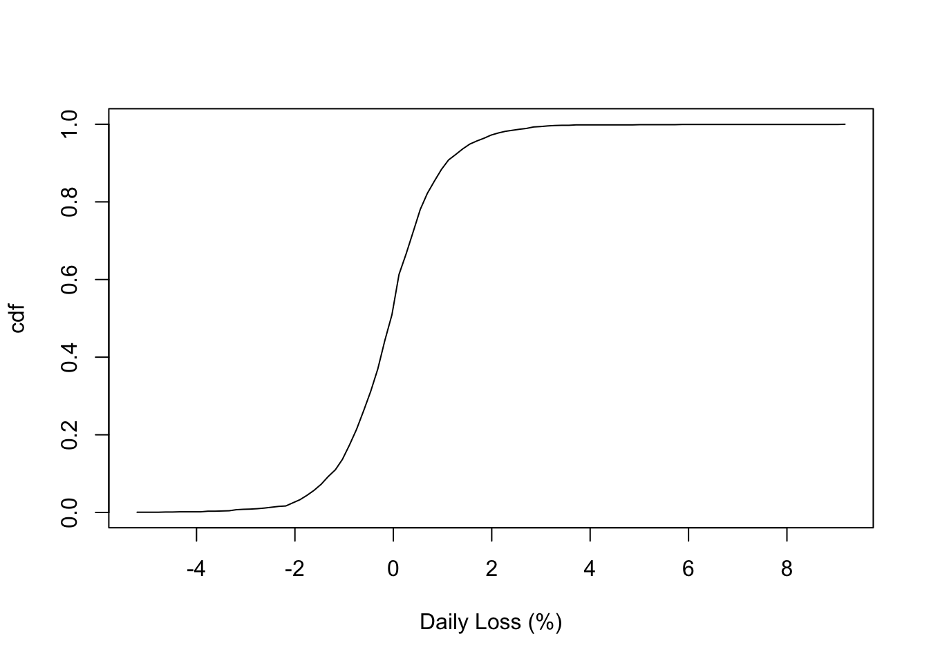
First, let’s focus on the DAX stock index. Fit an empirical distribution like last time (notice I’m using a data mask¹ in dst_empirical() this time).

# Fit an empirical distribution to the DAX stock index.
dax <- dst_empirical(DAX, data = stocks)
# Inspect the CDF.
plot(dax, xlab = "Daily Loss (%)")

You can easily calculate some standard quantiles in tabular format so that the inputs are placed alongside the calculated outputs: just use the enframe_ prefix instead of eval_ as we did above with the Null distribution.

enframe_quantile(dax, at = c(0.25, 0.5, 0.75), arg_name = "prob")

# A tibble: 3 × 2
   prob quantile
  <dbl>    <dbl>
1  0.25  -0.638 
2  0.5   -0.0473
3  0.75   0.468 

Or, more to the point here – and appealing to probaverse’s soft spot for risk-focused work – you can calculate return levels (also known as “Value at Risk” in financial applications) for specific return periods. If you don’t know what these are, they are just fancy names for quantiles.

return_periods <- c(5, 50, 100, 200, 500)
enframe_return(
  dax, 
  at = return_periods,
  arg_name = "return_period",
  fn_prefix = "daily_loss_pct"
)

# A tibble: 5 × 2
  return_period daily_loss_pct
          <dbl>          <dbl>
1             5          0.621
2            50          2.17 
3           100          2.75 
4           200          3.08 
5           500          3.71 

The tabular output becomes even more powerful when inserted into a table of models, because it facilitates comparisons and trends. To demonstrate, build a model for each stock. First, lengthen the data for this task.

# Lengthen the data using tidyverse.
stocks2 <- pivot_longer(
  stocks,
  everything(), 
  names_to = "stock", 
  values_to = "daily_loss_pct"
)
# Inspect
stocks2

# A tibble: 7,436 × 2
   stock daily_loss_pct
   <chr>          <dbl>
 1 DAX            0.928
 2 SMI           -0.620
 3 CAC            1.26 
 4 FTSE          -0.679
 5 DAX            0.441
 6 SMI            0.586
 7 CAC            1.86 
 8 FTSE           0.488
 9 DAX           -0.904
10 SMI           -0.328
# ℹ 7,426 more rows

Build a model for each stock using a group_by + summarise workflow from the tidyverse (please excuse the current need to wrap the distribution in list()). Notice that distributions become table entries, indicated here by their class <dst>.

# Create an Empirical distribution for each stock.
models <- stocks2 |> 
  group_by(stock) |> 
  summarise(model = list(dst_empirical(daily_loss_pct)))
# Inspect
models

# A tibble: 4 × 2
  stock model 
  <chr> <list>
1 CAC   <dst> 
2 DAX   <dst> 
3 FTSE  <dst> 
4 SMI   <dst> 

Now you can use a tidyverse workflow to calculate tables of quantiles for each model, and expand them. In fact, this workflow is common enough that I’m considering adding a dedicated verb for it.

return_levels <- models |>
  mutate(
    df = map(
      model,
      enframe_return,
      at = return_periods,
      arg_name = "return_period",
      fn_prefix = "daily_loss_pct"
    )
  ) |>
  unnest(df) |>
  select(!model)
# Inspect
print(return_levels, n = Inf)

# A tibble: 20 × 3
   stock return_period daily_loss_pct
   <chr>         <dbl>          <dbl>
 1 CAC               5          0.757
 2 CAC              50          2.37 
 3 CAC             100          2.78 
 4 CAC             200          3.41 
 5 CAC             500          3.97 
 6 DAX               5          0.621
 7 DAX              50          2.17 
 8 DAX             100          2.75 
 9 DAX             200          3.08 
10 DAX             500          3.71 
11 FTSE              5          0.542
12 FTSE             50          1.58 
13 FTSE            100          2.05 
14 FTSE            200          2.31 
15 FTSE            500          2.87 
16 SMI               5          0.552
17 SMI              50          2.03 
18 SMI             100          2.52 
19 SMI             200          2.91 
20 SMI             500          3.55 

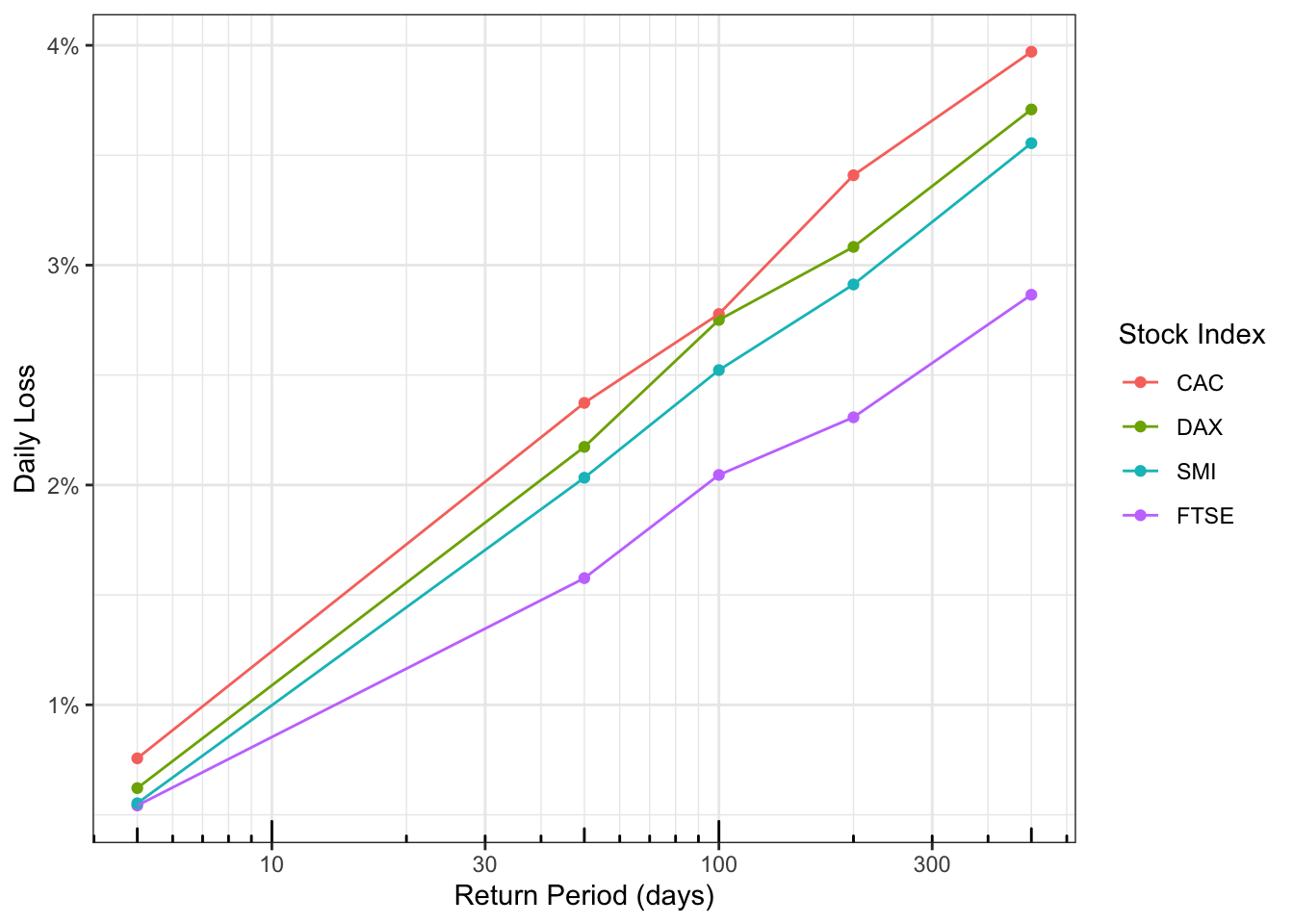
The result is a tidy dataset that’s ready for most analyses. For example, you can easily plot a comparison of the return levels of each stock. I make these plots all the time to facilitate risk-informed decision-making.

return_levels |> 
  mutate(stock = fct_reorder2(stock, return_period, daily_loss_pct)) |>
  ggplot(aes(return_period, daily_loss_pct, colour = stock)) +
  geom_point() +
  geom_line() +
  theme_bw() +
  scale_x_log10(
    "Return Period (days)",
    minor_breaks = c(1:10, 1:10 * 10, 1:10 * 100)
  ) +
  scale_y_continuous("Daily Loss", label = scales::label_number(suffix = "%")) +
  annotation_logticks(side = "b") +
  scale_colour_discrete("Stock Index")

🔗 Feature 3: make the distribution you need

You can create your own distributions with distionary by specifying only a minimal set of properties; all other properties are derived automatically and can be retrieved when needed.

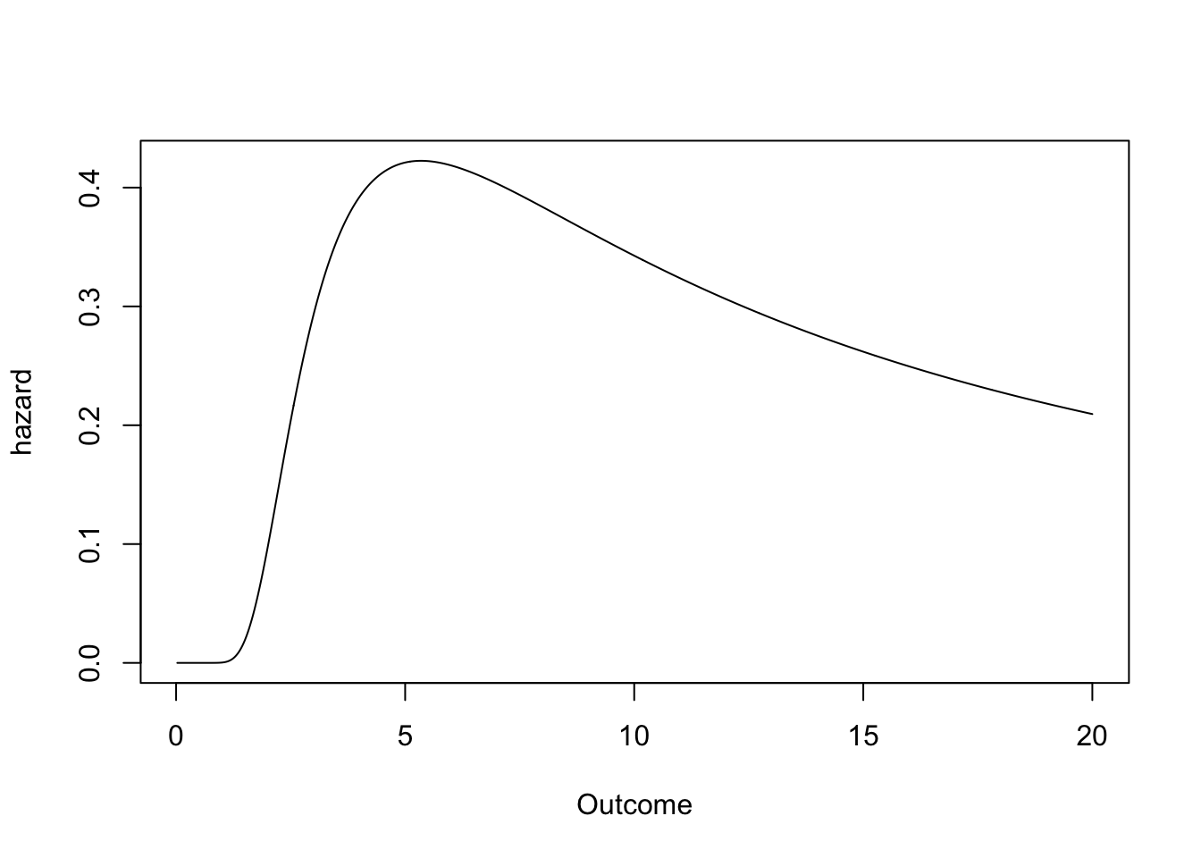
Let’s say you need an Inverse Gamma distribution but it’s not available in distionary. Currently, distionary assumes you’ll at least provide the density and CDF; you could retrieve these from the extraDistr package (functions dinvgamma() and pinvgamma()). Plug them into distionary’s distribution() function and enjoy access to a variety of properties you didn’t specify, like the mean, variance, skewness, and hazard function.

# Make an Inverse Gamma distribution (minimal example).
ig <- distribution(
  density = function(x) extraDistr::dinvgamma(x, alpha = 5, beta = 20),
  cdf = function(x) extraDistr::pinvgamma(x, alpha = 5, beta = 20),
  .vtype = "continuous",
)
# Calculate anything.
mean(ig)

[1] 5

variance(ig)

[1] 8.333333

skewness(ig)

[1] 3.464085

plot(ig, "hazard", to = 20, n = 1000, xlab = "Outcome")

You might also consider giving the distribution a .name – it pays off when you’re juggling multiple models. Adding .parameters provides additional specificity to the distribution .name, but are otherwise not yet used for functional purposes.

Here is a more complete implementation of the Inverse Gamma distribution, this time implemented as a function of the two parameters. Notice I also check that the parameters are positive (cheers to the checkmate package).

dst_invgamma <- function(alpha, beta) {
  checkmate::assert_number(alpha, lower = 0)
  checkmate::assert_number(beta, lower = 0)
  distribution(
    density = \(x) extraDistr::dinvgamma(x, alpha = alpha, beta = beta),
    cdf = \(x) extraDistr::pinvgamma(x, alpha = alpha, beta = beta),
    quantile = \(p) extraDistr::qinvgamma(p, alpha = alpha, beta = beta),
    random = \(n) extraDistr::rinvgamma(n, alpha = alpha, beta = beta),
    .name = "Inverse Gamma",
    .parameters = list(alpha = alpha, beta = beta),
    .vtype = "continuous",
  )
}

Now we can make that same Inverse Gamma distribution as before:

ig2 <- dst_invgamma(5, 20)
# Inspect
ig2

Inverse Gamma distribution (continuous) 
--Parameters--
alpha  beta 
    5    20 

By the way, this feature – being able to inspect other distribution properties even when they are not specified – is great for learning about probability. That’s because you can see the many ways distributions can be represented, not just by the usual density or probability mass functions seen in textbooks.

This feature also allows for extensibility of the probaverse. For example, the probaverse’s distplyr package creates mixture distributions, which do not have an explicit formula for the quantile function. However, this is not problematic – the distribution can still be defined, and distionary will figure out what the quantiles are.

🔗 What’s to come?

Currently, the distionary package provides key functionality to define and evaluate distribution objects. Future goals include:

• Broader coverage. Extending beyond univariate continuous distributions so mixed discrete/continuous and multivariate use cases feel first-class.
• Risk-native metrics. Making cost functions, tail expectations, and other decision metrics evaluate more naturally.
• Workflow ergonomics. Relaxing the requirement to supply density/CDF pairs and adding verbs that streamline common mutate-map-unnest patterns.

If this excites you, join the conversation by opening an issue or contributing.

Special thanks to the rOpenSci reviewers Katrina Brock and Christophe Dutang for insightful comments that improved this package. Also thanks to BGC Engineering Inc., the R Consortium, and the European Space Agency together with the Politecnico di Milano for supporting this project.