
Monday, August 10, 2026 From rOpenSci (https://ropensci.org/blog/2026/08/10/analisis-demografico-con-arcenso/). Except where otherwise noted, content on this site is licensed under the CC-BY license.
Population censuses are a key source of information for understanding the composition of populations and how they change across regions within a country. They provide essential evidence for research, the design and evaluation of public policies, and informed decision-making.
Working with census data typically involves several preliminary steps: identifying what information is available, downloading the data, organizing it, and preparing it for analysis. When this information is scattered across multiple sources and provided in different formats, the process can become complex.

ARcenso blog homepage
ARcenso is an R package developed as part of the rOpenSci Champions Program to facilitate access to Argentine census data and simplify its analysis.
In this article, the ARcenso development team demonstrates how to work with the historical census data available through the package in a simple, reproducible way.
The goal is to conduct a demographic analysis using official national data from the 1970 and 1980 censuses, combining visualisations and tables to explore the structure of the population—that is, how it is distributed by age and sex. This type of analysis helps characterise demographic changes over time, providing key information for research and the design of public policies.
🔗 Getting started
To run the code examples from this article on your own computer, make sure you have the following packages installed:
# If you don't have pak installed
install.packages("pak")

# Install ARcenso from GitHub
pak::pkg_install("soyandrea/arcenso")

# Install the required packages from CRAN
install.packages(c("dplyr", "tidyr", "ggplot2", "gt"))
Next, we load the packages needed to work with the census data and build indicators for the analysis:
library(arcenso)   # access census data
library(dplyr)     # data manipulation
library(tidyr)     # data tidying and transformation
library(ggplot2)   # data visualisation
library(gt)        # table formatting
🔗 Accessing census data
Now that the required packages are installed and loaded, we can use ARcenso to access census data from the 1970 and 1980 censuses. The package allows users to retrieve information by census year, topic, and geographic area of interest, using the official geographic codes defined by the National Institute of Statistics and Censuses (INDEC) of Argentina .
The check_repository() function helps identify the datasets available in the package. The topic argument specifies the subject of interest (for example, population structure), while geo_code identifies the geographic area.
If you are unsure which values are available for these arguments, you can explore the package metadata. The geo_metadata object contains the available geographic areas and their corresponding codes, while census_metadata provides information about the topics and tables included in the package.
In this example, we use population structure data (topic = "estructura") for the entire country (geo_code = "00"). As a first step, we use check_repository() to see which datasets are available.
check_repository(topic = "estructura", geo_code = "00")
# A tibble: 4 × 3
  id_cuadro              anio titulo
  <chr>                 <dbl> <chr>
1 1970_00_estructura_01  1970 Cuadro 1. Total del país. Población total, por gr…
2 1980_00_estructura_01  1980 Cuadro G3. Centros urbanos según tamaño y poblaci…
3 1980_00_estructura_02  1980 Cuadro G1. Total del país. Población total según …
4 1980_00_estructura_03  1980 Cuadro G2. Total del país. Población según sexo y…
The output of check_repository() lists the available years for the selected combination of topic and geographic area, together with the corresponding table identifiers (IDs) and their titles. Based on this information, we select the tables 1970_00_estructura_01 and 1980_00_estructura_03, which contain tabulations of the country’s total population by sex and age group and will be used throughout this analysis.
Tip: You can also explore the available data interactively using
arcenso_app(). Once you find the table you need, simply copy its ID and use it in your analysis.
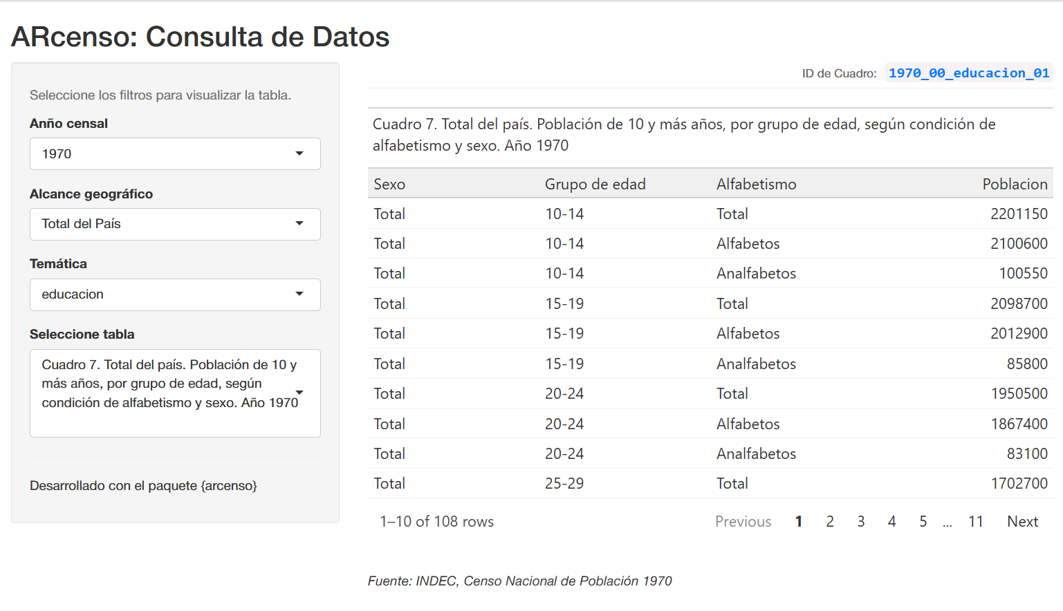
Interactive census data explorer with arcenso_app()
🔗 Data preparation
Once the tables of interest have been identified, we use get_census() to import them directly into the R session using their table identifiers.
As the structures of the two tables are not identical, we perform a series of transformations to harmonise the variables and create a consistent basis for comparison across censuses. In particular, we recode the age categories into five-year groups to ensure a common structure and add a column identifying the census year.
🔗 1970 Census
For the 1970 census, the data are already grouped into five-year age groups, so we only need to adjust the format of some labels and keep the variables relevant to the analysis.
# Country Total
poblacion_1970 <- get_census(id = "1970_00_estructura_01")

pob_1970 <- poblacion_1970 |>
  filter(sexo != "Total") |>
  mutate(
    censo = 1970,
    grupo_de_edad = case_when(
      grupo_de_edad == "0-4" ~ "00-04",
      grupo_de_edad == "5-9" ~ "05-09",
      TRUE ~ grupo_de_edad
    )
  ) |>
  rename(grupo_edad = grupo_de_edad) |>
  select(censo, sexo, grupo_edad, poblacion)
🔗 1980 Census
In contrast, the 1980 census table reports age as single years and includes additional information that is not relevant to this analysis. We therefore select the categories of interest and aggregate the data into five-year age groups to make them comparable with the 1970 census.
poblacion_1980 <- get_census(id = "1980_00_estructura_03")

pob_1980 <- poblacion_1980 |>
  filter(urbano_rural == "Total", sexo != "Total", edad != "Total") |>
  mutate(
    censo = 1980,
    edad_num = ifelse(edad == "85 y más", 85, as.numeric(edad)),
    grupo_edad = case_when(
      edad_num %in% c(0:4) ~ "00-04",
      edad_num %in% c(5:9) ~ "05-09",
      edad_num %in% c(10:14) ~ "10-14",
      edad_num %in% c(15:19) ~ "15-19",
      edad_num %in% c(20:24) ~ "20-24",
      edad_num %in% c(25:29) ~ "25-29",
      edad_num %in% c(30:34) ~ "30-34",
      edad_num %in% c(35:39) ~ "35-39",
      edad_num %in% c(40:44) ~ "40-44",
      edad_num %in% c(45:49) ~ "45-49",
      edad_num %in% c(50:54) ~ "50-54",
      edad_num %in% c(55:59) ~ "55-59",
      edad_num %in% c(60:64) ~ "60-64",
      edad_num %in% c(65:69) ~ "65-69",
      edad_num %in% c(70:74) ~ "70-74",
      edad_num %in% c(75:79) ~ "75-79",
      edad_num %in% c(80:84) ~ "80-84",
      TRUE ~ "85 y más"
    )
  ) |>
  select(censo, sexo, grupo_edad, poblacion)
🔗 Building the integrated database
Once both tables have been processed, we combine them into a single dataset and define the final structure of the variables, preparing the data for visualisation and the analysis of demographic indicators.
# We combine both geographic areas and prepare the variables for use
poblacion <-
  bind_rows(
    pob_1970,
    pob_1980
  ) |>
  mutate(
    poblacion = as.numeric(poblacion),
    sexo = factor(sexo, levels = c("Varones", "Mujeres")),
    grupo_edad = factor(
      grupo_edad,
      levels = c(
        "00-04",
        "05-09",
        "10-14",
        "15-19",
        "20-24",
        "25-29",
        "30-34",
        "35-39",
        "40-44",
        "45-49",
        "50-54",
        "55-59",
        "60-64",
        "65-69",
        "70-74",
        "75-79",
        "80-84",
        "85 y más"
      )
    )
  )
🔗 Population structure
Now that we have a dataset combining both censuses, with population totals organised by census year, sex, and age group, we can consistently compare the population composition across the two census years.
head(poblacion)


    # A tibble: 6 × 4
      censo sexo    grupo_edad poblacion
      <dbl> <fct>   <fct>          <dbl>
    1  1970 Varones 00-04        1196950
    2  1970 Mujeres 00-04        1158350
    3  1970 Varones 05-09        1163050
    4  1970 Mujeres 05-09        1133950
    5  1970 Varones 10-14        1114300
    6  1970 Mujeres 10-14        1086850
Organising the population by sex and five-year age groups allows us to analyse its structure using a variety of visualisations. In this case, we use a population pyramid, which makes it easier to interpret both dimensions together.
🔗 Population pyramid
A population pyramid displays the distribution of the population by age and sex simultaneously, typically showing males on the left and females on the right. By representing the proportion of people in each five-year age group, it provides a clear visual summary of the population structure.
In this case, we calculated the relative distribution of the population within each census, allowing us to compare the population structure between 1970 and 1980 regardless of total population size. The shape of the pyramid also allows us to identify broad demographic patterns, such as a higher concentration of younger age groups or a relatively older population profile.
We then calculated the relative distribution of the population in each census and constructed a population pyramid to compare the population structure of the two censuses.
# Dataset for the Population Pyramid
piramide <- poblacion |>
  group_by(censo, sexo) |>
  mutate(
    poblacion_rel = if_else(
      sexo == "Varones",
      -poblacion / sum(poblacion),
      poblacion / sum(poblacion)
    )
  ) |>
  ungroup()

# Comparison Pyramid
piramide |>
  ggplot(aes(x = poblacion_rel, y = grupo_edad, fill = sexo)) +
  geom_col() +
  facet_wrap(~censo, ncol = 2) +
  scale_fill_manual(values = c("#00f59b", "#7014f2")) +
  scale_x_continuous(
    labels = function(x) paste0(abs(round(x * 100, 1)), "%"),
    limits = c(-0.15, 0.15),
    breaks = seq(-0.15, 0.15, by = 0.05)
  ) +
  labs(
    title = "Gráfico 1. Estructura de la población por sexo y grupo quinquenal de edad.",
    subtitle = "Argentina. Años 1970 y 1980",
    x = "Porcentaje",
    y = "Grupo quinquenal de edad",
    caption = "Fuente: INDEC, Censo Nacional de Población 1970 y 1980. Procesado con ARcenso.",
    fill = "Sexo"
  ) +
  theme_bw() +
  theme(
    legend.position = "bottom",
    strip.text = element_text(face = "bold", size = 12)
  )
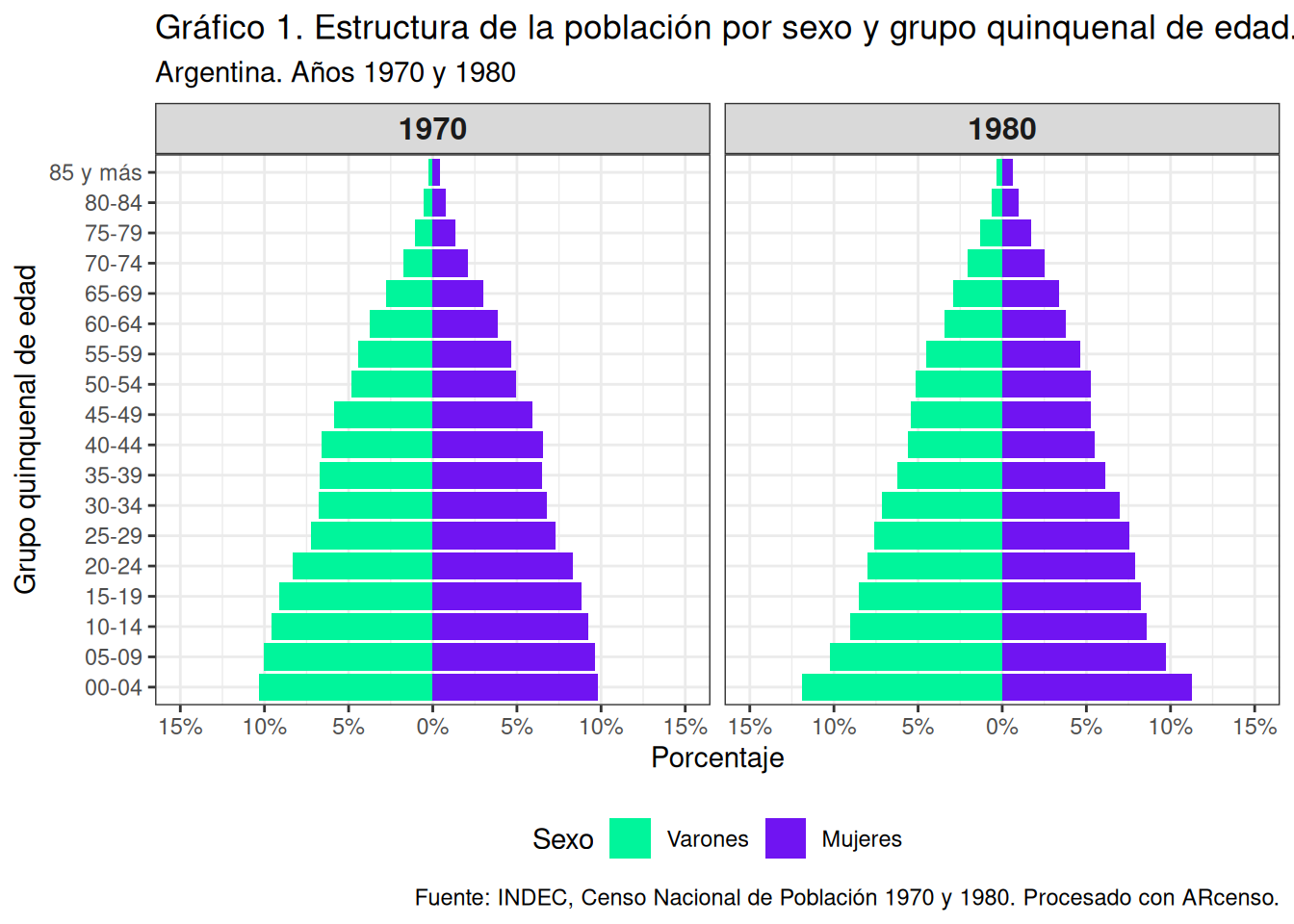
Figure 1. Population structure by sex and five-year age group. Argentina. Year 1970 and 1980. Source: INDEC, Censo Nacional de Población 1970 y 1980. Processed with ARcenso.
Both censuses show a young population structure, with a high concentration of people in the younger age groups. However, by 1980, a slight shift towards the adult age groups is already apparent, suggesting the early stages of population aging.
🔗 Construction of demographic indicators
While the population pyramid provides an overall view of the population structure, demographic indicators offer summary measures that allow these patterns to be quantified and compared more precisely. In this section, we calculate two commonly used indicators to complement the visual analysis.
🔗 Aging index
The aging index compares the number of older adults (aged 65 years and over) with the number of children (aged 0–14 years). It provides a simple way to see whether the population is weighted more toward younger age groups or older age groups.
envejecimiento <- poblacion |>
  group_by(censo) |>
  summarise(
    poblacion_0a14 = sum(poblacion[
      grupo_edad %in% c("00-04", "05-09", "10-14")
    ]),
    poblacion_65ymas = sum(poblacion[
      grupo_edad %in% c("65-69", "70-74", "75-79", "80-84", "85 y más")
    ]),
    indice = round(poblacion_65ymas / poblacion_0a14 * 100, 0)
  )


gt(envejecimiento) |>
  tab_header(
    title = "Comparación del índice de envejecimiento",
    subtitle = "Argentina. Años 1970 y 1980"
  ) |>
  tab_spanner(
    label = "Población",
    columns = c(poblacion_0a14, poblacion_65ymas)
  ) |>
  fmt_number(
    columns = c(poblacion_0a14, poblacion_65ymas),
    decimals = 0,
    sep_mark = "."
  ) |>
  cols_label(
    poblacion_0a14 = "0 a 14 años",
    poblacion_65ymas = "65 años y más",
    indice = "Indice"
  ) |>
  tab_source_note(
    source_note = md(
      "**Fuente:** elaboración propia en base a datos de INDEC (Censos Nacionales de Población 1970 y 1980)."
    )
  )
| Aging Index Comparison | |||
| Argentina. 1970s and 1980s | |||
| Census | Population | Index | |
|---|---|---|---|
| Ages 0 to 14 | 65 years and older | ||
| 1970 | 6,853,450 | 1,631,400 | 24 |
| 1980 | 8,480,768 | 2,290,564 | 27 |
| Source: Author’s own calculations based on INDEC data (1970 and 1980 National Population Censuses). | |||
The increase in the aging index reflects a change in the population age structure between 1970 and 1980, indicating a larger relative share of people aged 65 years and over compared with the younger population. This suggests a gradual aging of the population.
🔗 Female-to-Male ratio
This indicator shows how many women there are for every 100 men in a specific population group. Here, we calculate it for people aged 60 years and over, where differences between women and men tend to become more pronounced.
feminidad <- poblacion |>
  filter(
    grupo_edad %in% c("60-64", "65-69", "70-74", "75-79", "80-84", "85 y más")
  ) |>
  group_by(censo, grupo_edad, sexo) |>
  summarise(poblacion = sum(poblacion), .groups = "drop") |>
  pivot_wider(names_from = sexo, values_from = poblacion) |>
  mutate(
    indice_feminidad = round(Mujeres / Varones * 100, 0)
  ) |>
  select(-Varones, -Mujeres)


feminidad_plot <- feminidad |>
  pivot_wider(
    names_from = censo,
    values_from = indice_feminidad,
    names_prefix = "censo_"
  ) |>
  ggplot(aes(y = grupo_edad)) +
  geom_segment(
    aes(x = censo_1970, xend = censo_1980, yend = grupo_edad),
    color = "grey85",
    linewidth = 1
  ) +
  geom_point(
    aes(x = censo_1970),
    color = "#ff0f7b",
    size = 3
  ) +
  geom_point(
    aes(x = censo_1980),
    color = "#f89b29",
    size = 3
  ) +
  geom_text(
    aes(x = censo_1970, label = censo_1970),
    hjust = 1.4,
    size = 3
  ) +
  geom_text(
    aes(x = censo_1980, label = censo_1980),
    hjust = -0.4,
    size = 3
  ) +
  labs(
    x = "Mujeres por cada 100 varones",
    y = "Grupo de edad",
    title = "Cambio en el índice de feminidad de la población de 60 años y más",
    subtitle = "Argentina, Años 1970 y 1980",
    caption = "Fuente: INDEC, Censo Nacional de Población 1970 y 1980. Procesado con ARcenso."
  ) +
  theme_minimal()

feminidad_plot
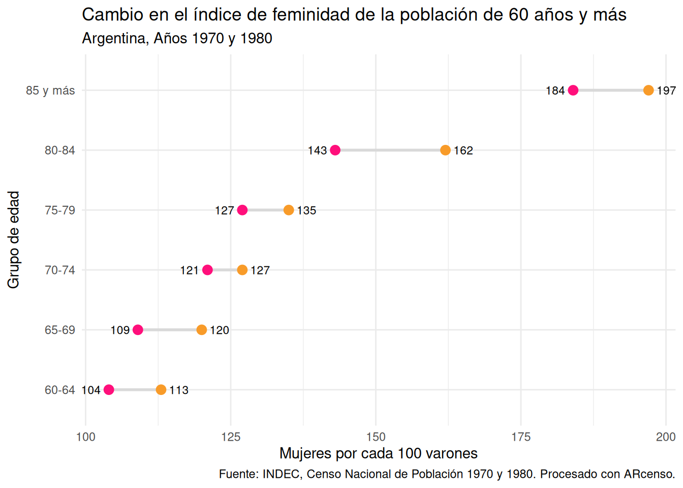
Change in the female-to-male ratio among the population aged 60 and older. Argentina. Year 1970 and 1980. Source: INDEC, Censo Nacional de Población 1970 y 1980. Processed with ARcenso.
The female-to-male ratio shows a higher proportion of women in the older age groups. This difference becomes more pronounced between 1970 and 1980 across all the age groups analysed, reflecting patterns of higher female life expectancy.
🔗 What does this analysis tell us?
In demographic analysis, the most time-consuming part is often not calculating indicators or creating visualisations, but the work that comes beforehand: identifying the available data for each census, understanding how it is organised, and building a consistent framework that enables comparisons across census years.
In this example, that process involved locating the relevant tables, understanding the structural differences between the 1970 and 1980 censuses, and harmonising the variables based on the available information to create a comparable dataset. This is precisely what ARcenso is designed to simplify. The check_repository() function helps identify the available tables, get_census() imports the data into R in a structured format, and arcenso_app() provides an interactive way to explore the repository.
Once the data have been organised, the analysis becomes more accessible, reproducible, and easier to extend to new questions.
ARcenso is still a work in progress. Future developments will incorporate additional census years and continue expanding the package’s analytical capabilities. The package was created to make Argentine census data easier to discover, access, and analyse, while building on the collaborative efforts of the open-source community.
If you would like to explore further,check out the vignettes in the package, which include additional examples to work with census data.
Filed under
Suggest an edit
Open a pull request
