Tuesday, December 5, 2017 From rOpenSci (https://ropensci.org/blog/2017/12/05/magick-16/). Except where otherwise noted, content on this site is licensed under the CC-BY license.
This week magick 1.6 appeared on CRAN. This release is a big all-round maintenance update with lots of tweaks and improvements across the package.
The NEWS file gives an overview of changes in this version. In this post we highlight some changes.
library(magick)
stopifnot(packageVersion('magick') >= 1.6)
If you are new to magick, check out the vignette for a quick introduction.
🔗 Perfect Graphics Rendering
I have fixed a few small rendering imperfections in the graphics device. The native magick graphics device image_graph() now renders identical or better quality images as the R-base bitmap devices png, jpeg, etc.
One issue was that sometimes magick graphics would show a 1px black border around the image. It turned out this is caused by rounding of clipping coordinates.
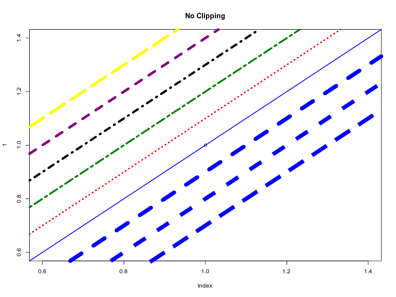
When R calculates clipping area it often ends up at non-whole values. It is then up to the graphics device to decide what to do with the pixel that is partially clipped. Let’s show clipping in action:
testplot <- function(title = ""){
  plot(1, main = title)
  abline(0, 1, col = "blue", lwd = 2, lty = "solid")
  abline(0.1, 1, col = "red", lwd = 3, lty = "dotted")
  abline(0.2, 1, col = "green", lwd = 4, lty = "twodash")
  abline(0.3, 1, col = "black", lwd = 5, lty = "dotdash")
  abline(0.4, 1, col = "purple", lwd = 6, lty = "dashed")
  abline(0.5, 1, col = "yellow", lwd = 7, lty = "longdash")
  abline(-0.1, 1, col = "blue", lwd = 10, lend = "round", lty = "dashed")
  abline(-0.2, 1, col = "blue", lwd = 10, lend = "butt", lty = "dashed")
  abline(-0.3, 1, col = "blue", lwd = 10, lend = "square", lty = "dashed")
}
Now we run it with and without clipping:
img2 <- magick::image_graph(clip = FALSE)
testplot("Without clipping")
dev.off()
img1 <- magick::image_graph(clip = TRUE)
testplot("With clipping")
dev.off()
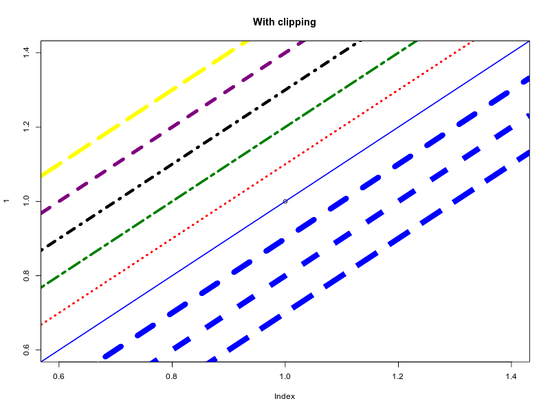
As we can see the latter image is now perfectly clipped. The colored lines are truncated exactly at the pixel where the axis starts. This is not always the case in base R ;)
🔗 Font Families
In magick there are two ways to render text on an image. You can either open the image or graphic in the magick graphics device and then use base R text() function to print text. Alternatively there is image_annotate() which is a simpler version to print some text on an image.
Wherever text rendering is involved, two major headache arise: encoding and fonts. The latter is tricky because different operating systems have different fonts with different names. In addition a font can be specified as a name, or family name, or alias.
Below is a simple test that I use to quickly inspect if fonts are working on different systems:
img <- image_graph(width = 800, height = 500, pointsize = 20, res = 96)
graphics::plot.new()
graphics::par(mar = c(0,0,3,0))
graphics::plot.window(xlim = c(0, 20), ylim = c(-.5, 8))
title(expression(Gamma %prop% sum(x[alpha], i==1, n) * sqrt(mu)), expression(hat(x)))

# Standard families as supported by other devices
text(0.95, 7, "abcdefg  - Helvetica", pos = 4, family = "helvetica")
text(0.95, 6, "abcdefg  - Sans (Arial)", pos = 4, family = "sans")
text(0.95, 5, "abcdefg - Serif (Times)", pos = 4, family = "serif")
text(0.95, 4, "abcdefg - Monospace (Courier New)", pos = 4, family = "mono")
text(0.95, 3, "abcdefg - Symbol Face", pos = 4, font = 5)
text(0.95, 2, "abcdefg  - Comic Sans", pos = 4, family = "Comic Sans")
text(0.95, 1, "abcdefg - Georgia Serif", pos = 4, family = "Georgia")
text(0.95, 0, "abcdefg - Courier", pos = 4, family = "Courier")
dev.off()
img <- image_border(img, 'red', geometry = '2x2')
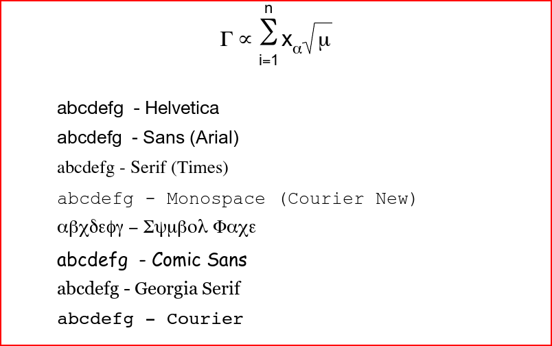
R requires that a graphics device supports at least 4 font types: serif, sans, mono and symbol. The latter is a special 8bit font with some Greek letters and other characters needed for rendering math. This set of fonts corresponds to the original 13 base fonts from the 1984 postscript standard:
- 4x Courier (Regular, Oblique, Bold, Bold Oblique)
- 4x Helvetica (Regular, Oblique, Bold, Bold Oblique)
- 4x Times (Roman, Italic, Bold, Bold Italic)
- Symbol
Below a photo of the 1985 Apple Laser Writer which was the first laser printer to use the PostScript language and support all these fonts! Not much later PostScript graphics devices were adopted by R’s predecessor “The New S” (The New S Language, 1988).

🔗 Geometry Helpers
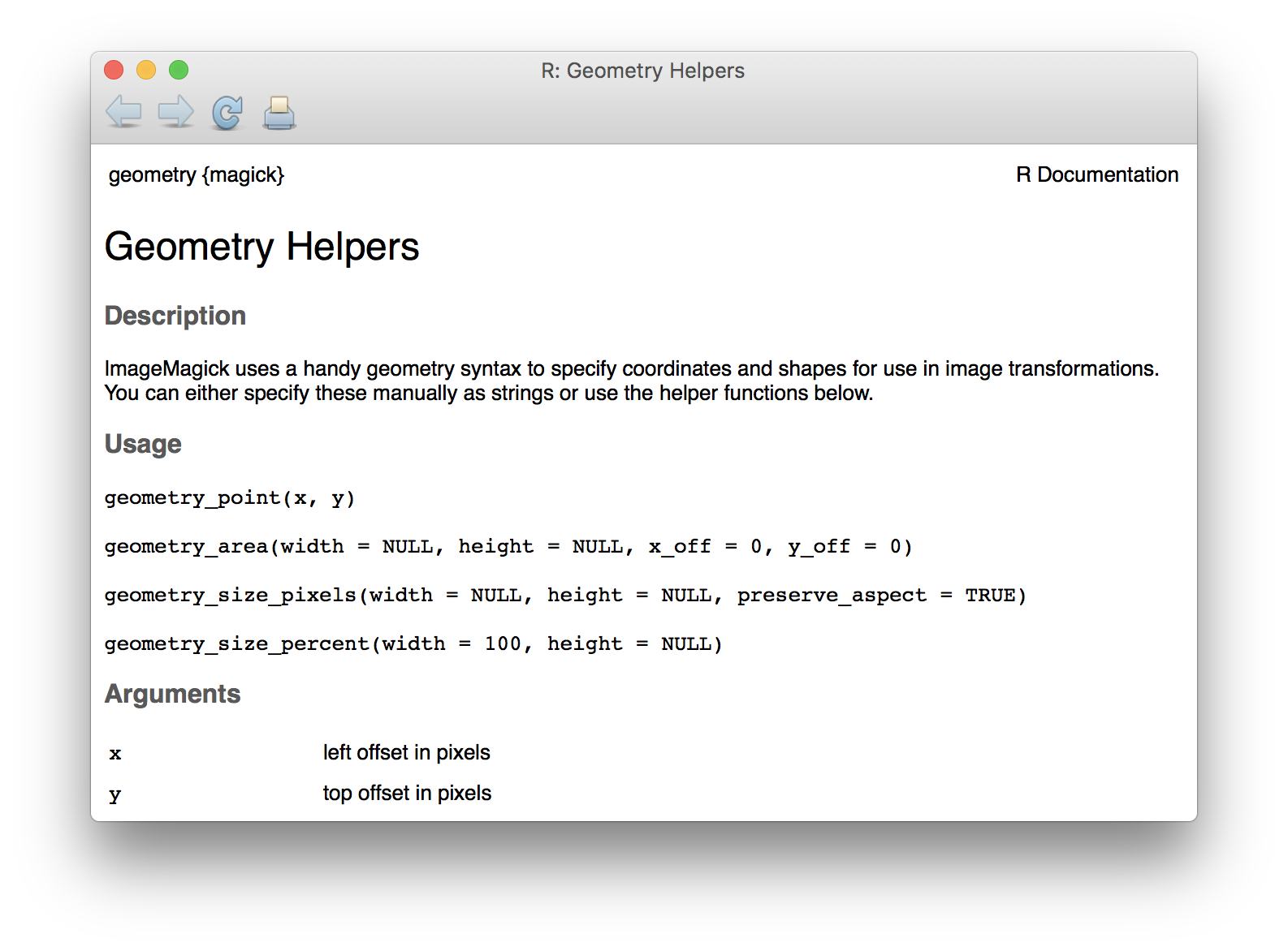
Another major improvement in this release is the introduction of helper functions for geometry and option strings. Many functions in magick require a special geometry syntax to specify a size, area, or point. For example to resize an image you need to specify a size:
image_resize(img, "50%")
image_resize(img, "300x300")
image_resize(img, "300x300!")
Or to crop you need to specify an area which consists of a size and offset:
image_crop(img, "300x300+100+100")
We added a few handy ?geometry helper functions to generate proper geometry syntax
🔗 Magick Options
A lot of the power in ImageMagick is contained in the hundreds of built-in filters, colorspaces, compose operators, disposal types, convolution kernels, noise types and what not. These are specified simply as a string in the function.
For example in our previous post about Image Convolution we discussed a few kernel types:
# Gaussian Kernel
img %>% image_convolve('Gaussian:0x5', scaling = '60,40%')

# Sobel Kernel
img %>% image_convolve('Sobel')

# Difference of Gaussians
img %>% image_convolve('DoG:0,0,2')
Supported values for each option are described in the online ImageMagick documentation. We now have added functions in the magick package that list all values for each option. This should make it a easier to see what is supported and harness the full power of built-in ImageMagick algorithms.
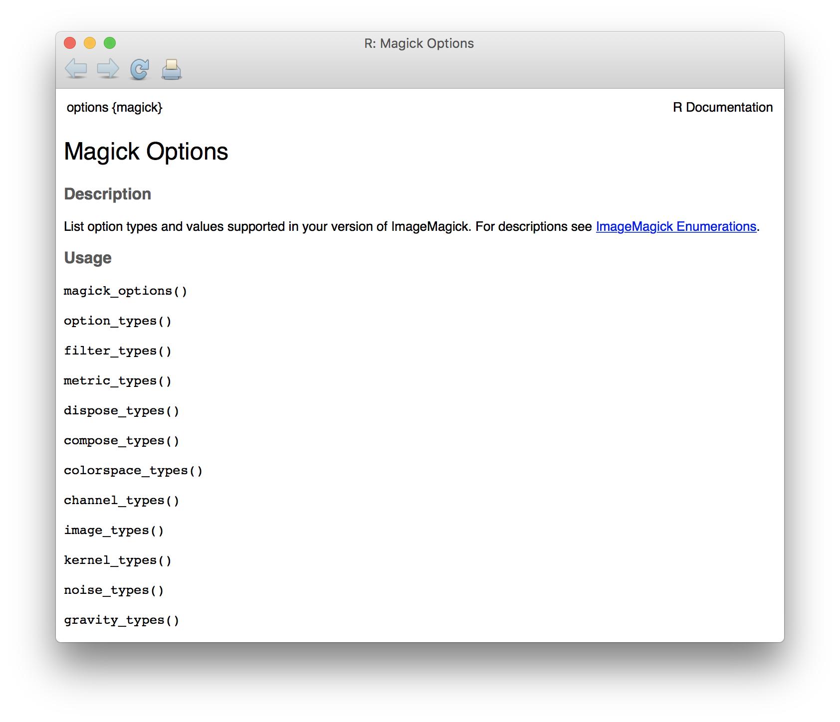
So we can now easily list e.g. supported kernel types:
> kernel_types()
 [1] "Undefined"     "Unity"         "Gaussian"      "DoG"
 [5] "LoG"           "Blur"          "Comet"         "Binomial"
 [9] "Laplacian"     "Sobel"         "FreiChen"      "Roberts"
[13] "Prewitt"       "Compass"       "Kirsch"        "Diamond"
[17] "Square"        "Rectangle"     "Disk"          "Octagon"
[21] "Plus"          "Cross"         "Ring"          "Peaks"
[25] "Edges"         "Corners"       "Diagonals"     "ThinDiagonals"
[29] "LineEnds"      "LineJunctions" "Ridges"        "ConvexHull"
[33] "ThinSe"        "Skeleton"      "Chebyshev"     "Manhattan"
[37] "Octagonal"     "Euclidean"     "User Defined"
That’s a lot of kernels.
🔗 Fuzz Scaling
Finally one more (breaking) change: several functions in magick use a fuzz parameter to specify the max distance between two colors to be considered similar.
For example the flood fill algorithm (the paint-bucket button in ms-paint) changes the color of a given starting pixel, and then recursively all adjacent pixels that have the same color. However sometimes neighboring pixels are not precisely the same color, but nearly the same. The fuzz parameter allows the fill to continue when pixels are not the same but similar color.
# Paint the shirt orange
frink <- image_read("https://jeroen.github.io/images/frink.png") %>%
  image_fill("orange", point = "+100+200", fuzz = 25)

What has changed in this version is that fuzz parameter been rescaled to a percentage. Hence you should always provide a value between 0 and 100. Previously it was the absolute distance between colors, but this depends on the type and color depth of the image at hand, which was very confusing.

