
Friday, September 6, 2019 From rOpenSci (https://ropensci.org/blog/2019/09/06/ucscxenatools-surv/). Except where otherwise noted, content on this site is licensed under the CC-BY license.
The UCSC Xena platform provides an unprecedented resource for public omics data from big projects like The Cancer Genome Atlas (TCGA), however, it is hard for users to incorporate multiple datasets or data types, integrate the selected data with popular analysis tools or homebrewed code, and reproduce analysis procedures. To address this issue, we developed an R package UCSCXenaTools for enabling data retrieval, analysis integration and reproducible research for omics data from the UCSC Xena platform1.
In this technote we will outline how to use the UCSCXenaTools package to pull gene expression and clinical data from UCSC Xena for survival analysis.
For general usage of UCSCXenaTools, please refer to the package vignette. Any bug or feature request can be reported in GitHub issues.
🔗 Installation
UCSCXenaTools is available from CRAN:
install.packages("UCSCXenaTools")
Alternatively, the latest development version can be downloaded from GitHub:
remotes::install_github("ropensci/UCSCXenaTools", build_vignettes = TRUE, dependencies = TRUE)
🔗 How it works
Before actually pulling data, understanding how UCSCXenaTools works (see Figure 1) will help users locate the most important function to use.
Generally,
- for operating datasets, we use functions whose names start with
Xena - for operating subset of a dataset, we use functions whose names start with
fetch_
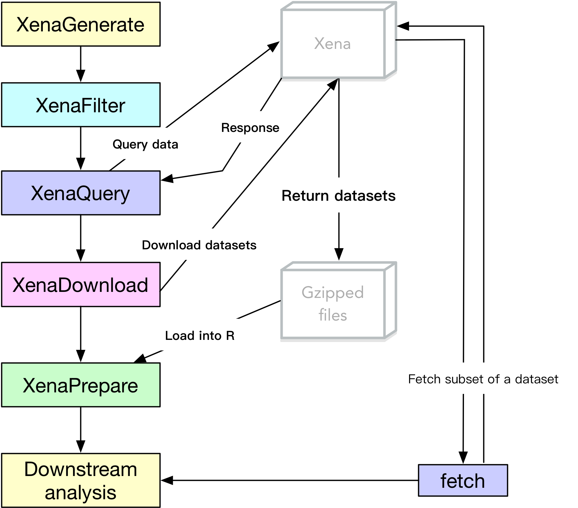 Figure 1. The UCSCXenaTools pipeline
We will provide an example illustrating how to use UCSCXenaTools to study the effect of expression of the KRAS gene on prognosis of Lung Adenocarcinoma (LUAD) patients. KRAS is a known driver gene in LUAD. We retrieve expression data for the KRAS gene and survival status data for LUAD patients from the TCGA and use these as input to a survival analysis, frequently used in cancer research.
🔗 Download data
First we get information on all datasets in the TCGA LUAD cohort and store as luad_cohort object.
suppressMessages(library(UCSCXenaTools))
suppressMessages(library(dplyr))
luad_cohort = XenaData %>%
  filter(XenaHostNames == "tcgaHub") %>% # select TCGA Hub
  XenaScan("TCGA Lung Adenocarcinoma")   # select LUAD cohort

luad_cohort
#> # A tibble: 27 x 17
#>    XenaHosts XenaHostNames XenaCohorts XenaDatasets SampleCount DataSubtype
#>    <chr>     <chr>         <chr>       <chr>        <chr>       <chr>
#>  1 https://… tcgaHub       TCGA Lung … RABIT/separ… 467         Transcript…
#>  2 https://… tcgaHub       TCGA Lung … RABIT/separ… 120         Transcript…
#>  3 https://… tcgaHub       TCGA Lung … TCGA.LUAD.s… 151         DNA methyl…
#>  4 https://… tcgaHub       TCGA Lung … TCGA.LUAD.s… 492         DNA methyl…
#>  5 https://… tcgaHub       TCGA Lung … TCGA.LUAD.s… 516         copy numbe…
#>  6 https://… tcgaHub       TCGA Lung … TCGA.LUAD.s… 543         somatic mu…
#>  7 https://… tcgaHub       TCGA Lung … TCGA.LUAD.s… 237         protein ex…
#>  8 https://… tcgaHub       TCGA Lung … TCGA.LUAD.s… 576         gene expre…
#>  9 https://… tcgaHub       TCGA Lung … TCGA.LUAD.s… 60          miRNA matu…
#> 10 https://… tcgaHub       TCGA Lung … TCGA.LUAD.s… 576         gene expre…
#> # … with 17 more rows, and 11 more variables: Label <chr>, Type <chr>,
#> #   AnatomicalOrigin <chr>, SampleType <chr>, Tags <chr>, ProbeMap <chr>,
#> #   LongTitle <chr>, Citation <chr>, Version <chr>, Unit <chr>,
#> #   Platform <chr>
🔗 Download clinical dataset
Now we download the clinical dataset of the TCGA LUAD cohort and load it into R.
cli_query = luad_cohort %>%
  filter(DataSubtype == "phenotype") %>%  # select clinical dataset
  XenaGenerate() %>%  # generate a XenaHub object
  XenaQuery() %>%
  XenaDownload()
#> This will check url status, please be patient.
#> All downloaded files will under directory /var/folders/mx/rfkl27z90c96wbmn3_kjk8c80000gn/T//Rtmp2ihvVq.
#> The 'trans_slash' option is FALSE, keep same directory structure as Xena.
#> Creating directories for datasets...
#> Downloading TCGA.LUAD.sampleMap/LUAD_clinicalMatrix.gz

cli = XenaPrepare(cli_query)

# See a few rows
head(cli)
#> # A tibble: 6 x 157
#>   sampleID ABSOLUTE_Ploidy ABSOLUTE_Purity AKT1  ALK_translocati… BRAF
#>   <chr>              <dbl>           <dbl> <chr> <chr>            <chr>
#> 1 TCGA-05…           NA              NA    <NA>  <NA>             <NA>
#> 2 TCGA-05…            3.77            0.46 none  <NA>             p.A7…
#> 3 TCGA-05…           NA              NA    <NA>  <NA>             <NA>
#> 4 TCGA-05…           NA              NA    none  <NA>             p.L6…
#> 5 TCGA-05…            2.04            0.48 none  <NA>             none
#> 6 TCGA-05…            3.29            0.48 none  <NA>             p.G4…
#> # … with 151 more variables: CBL <chr>, CTNNB1 <chr>,
#> #   Canonical_mut_in_KRAS_EGFR_ALK <chr>,
#> #   Cnncl_mt_n_KRAS_EGFR_ALK_RET_ROS1_BRAF_ERBB2_HRAS_NRAS_AKT1_MAP2 <chr>,
#> #   EGFR <chr>, ERBB2 <chr>, ERBB4 <chr>,
#> #   Estimated_allele_fraction_of_a_clonal_varnt_prsnt_t_1_cpy_pr_cll <dbl>,
#> #   Expression_Subtype <chr>, HRAS <chr>, KRAS <chr>, MAP2K1 <chr>,
#> #   MET <chr>, NRAS <chr>, PIK3CA <chr>, PTPN11 <chr>, Pathology <chr>,
#> #   Pathology_Updated <chr>, RET_translocation <chr>,
#> #   ROS1_translocation <chr>, STK11 <chr>,
#> #   WGS_as_of_20120731_0_no_1_yes <dbl>, `_EVENT` <dbl>,
#> #   `_INTEGRATION` <chr>, OS.time <dbl>, OS <dbl>, OS.unit <chr>,
#> #   `_PANCAN_CNA_PANCAN_K8` <chr>, `_PANCAN_Cluster_Cluster_PANCAN` <chr>,
#> #   `_PANCAN_DNAMethyl_LUAD` <chr>, `_PANCAN_DNAMethyl_PANCAN` <chr>,
#> #   `_PANCAN_RPPA_PANCAN_K8` <chr>, `_PANCAN_UNC_RNAseq_PANCAN_K16` <chr>,
#> #   `_PANCAN_miRNA_PANCAN` <chr>, `_PANCAN_mirna_LUAD` <chr>,
#> #   `_PANCAN_mutation_PANCAN` <chr>, `_PATIENT` <chr>, RFS.time <dbl>,
#> #   RFS <dbl>, RFS.unit <chr>, `_TIME_TO_EVENT` <dbl>,
#> #   `_TIME_TO_EVENT_UNIT` <chr>, `_cohort` <chr>,
#> #   `_primary_disease` <chr>, `_primary_site` <chr>,
#> #   additional_pharmaceutical_therapy <chr>,
#> #   additional_radiation_therapy <chr>,
#> #   additional_surgery_locoregional_procedure <chr>,
#> #   additional_surgery_metastatic_procedure <chr>,
#> #   age_at_initial_pathologic_diagnosis <dbl>,
#> #   anatomic_neoplasm_subdivision <chr>,
#> #   anatomic_neoplasm_subdivision_other <chr>, bcr_followup_barcode <chr>,
#> #   bcr_patient_barcode <chr>, bcr_sample_barcode <chr>,
#> #   days_to_additional_surgery_locoregional_procedure <dbl>,
#> #   days_to_additional_surgery_metastatic_procedure <dbl>,
#> #   days_to_birth <dbl>, days_to_collection <dbl>, days_to_death <dbl>,
#> #   days_to_initial_pathologic_diagnosis <dbl>,
#> #   days_to_last_followup <dbl>,
#> #   days_to_new_tumor_event_after_initial_treatment <dbl>,
#> #   disease_code <chr>, dlco_predictive_percent <dbl>,
#> #   eastern_cancer_oncology_group <dbl>, egfr_mutation_performed <chr>,
#> #   egfr_mutation_result <chr>, eml4_alk_translocation_method <chr>,
#> #   eml4_alk_translocation_performed <chr>,
#> #   followup_case_report_form_submission_reason <chr>,
#> #   followup_treatment_success <chr>, form_completion_date <chr>,
#> #   gender <chr>, histological_type <chr>,
#> #   history_of_neoadjuvant_treatment <chr>, icd_10 <chr>,
#> #   icd_o_3_histology <chr>, icd_o_3_site <chr>,
#> #   informed_consent_verified <chr>, initial_weight <dbl>,
#> #   intermediate_dimension <dbl>, is_ffpe <chr>,
#> #   karnofsky_performance_score <dbl>, kras_gene_analysis_performed <chr>,
#> #   kras_mutation_found <chr>, kras_mutation_result <chr>,
#> #   location_in_lung_parenchyma <chr>, longest_dimension <dbl>,
#> #   lost_follow_up <chr>, new_neoplasm_event_type <chr>,
#> #   new_tumor_event_after_initial_treatment <chr>,
#> #   number_pack_years_smoked <dbl>, oct_embedded <lgl>, other_dx <chr>,
#> #   pathologic_M <chr>, pathologic_N <chr>, pathologic_T <chr>,
#> #   pathologic_stage <chr>, pathology_report_file_name <chr>, …
🔗 Download KRAS gene expression
To download gene expression data, first we need to select the right dataset.
ge = luad_cohort %>%
  filter(DataSubtype == "gene expression RNAseq", Label == "IlluminaHiSeq")
ge
#> # A tibble: 1 x 17
#>   XenaHosts XenaHostNames XenaCohorts XenaDatasets SampleCount DataSubtype
#>   <chr>     <chr>         <chr>       <chr>        <chr>       <chr>
#> 1 https://… tcgaHub       TCGA Lung … TCGA.LUAD.s… 576         gene expre…
#> # … with 11 more variables: Label <chr>, Type <chr>,
#> #   AnatomicalOrigin <chr>, SampleType <chr>, Tags <chr>, ProbeMap <chr>,
#> #   LongTitle <chr>, Citation <chr>, Version <chr>, Unit <chr>,
#> #   Platform <chr>
Now we fetch KRAS gene expression values.
# You can pass gene symbols to 'identifiers' option
# to obtain their values in a dataset.
# A matrix will be returned by 'fetch_dense_values' function
# with rows corresponding to genes,
# so here we extract the first row.
KRAS = fetch_dense_values(host = ge$XenaHosts,
                          dataset = ge$XenaDatasets,
                          identifiers = "KRAS",
                          use_probeMap = TRUE) %>%
  .[1, ]
#> -> Checking identifiers...
#> -> use_probeMap is TRUE, skipping checking identifiers...
#> -> Done.
#> -> Checking samples...
#> -> Done.
#> -> Checking if the dataset has probeMap...
#> -> Done. ProbeMap is found.

head(KRAS)
#> TCGA-69-7978-01 TCGA-62-8399-01 TCGA-78-7539-01 TCGA-50-5931-11
#>           10.25           10.29           10.82           10.29
#> TCGA-73-4658-01 TCGA-44-6775-01
#>           10.36           10.03
🔗 Merge expression data and survival status
Next, we join the two data.frame by sampleID and keep necessary columns. Here we focus on ‘Primary Tumor’ for simplicity.
merged_data = tibble(sampleID = names(KRAS),
                     KRAS_expression = as.numeric(KRAS)) %>%
  left_join(cli, by = "sampleID") %>%
  filter(sample_type == "Primary Tumor") %>%  # Keep only 'Primary Tumor'
  select(sampleID, KRAS_expression, OS.time, OS) %>%
  rename(time = OS.time,
         status = OS)


head(merged_data)
#> # A tibble: 6 x 4
#>   sampleID        KRAS_expression  time status
#>   <chr>                     <dbl> <dbl>  <dbl>
#> 1 TCGA-69-7978-01           10.2    134      0
#> 2 TCGA-62-8399-01           10.3   2696      0
#> 3 TCGA-78-7539-01           10.8    791      0
#> 4 TCGA-73-4658-01           10.4   1600      1
#> 5 TCGA-44-6775-01           10.0    705      0
#> 6 TCGA-44-2655-01            9.75  1324      0
🔗 Survival analysis
To study the effect of KRAS gene expression on prognosis of LUAD patients, we show two approaches:
- use Cox model to determine the effect when KRAS gene expression increases
- use Kaplan-Meier curve and log-rank test to observe the difference in different ofKRAS gene expression status, i.e. high or low
We will use package survival and survminer to create models and plot survival curves, respectively.
library(survival)
library(survminer)
#> Loading required package: ggplot2
#> Loading required package: ggpubr
#> Loading required package: magrittr
🔗 Cox model
fit = coxph(Surv(time, status) ~ KRAS_expression, data = merged_data)
fit
#> Call:
#> coxph(formula = Surv(time, status) ~ KRAS_expression, data = merged_data)
#>
#>                   coef exp(coef) se(coef)     z      p
#> KRAS_expression 0.2927    1.3400   0.1020 2.871 0.0041
#>
#> Likelihood ratio test=7.67  on 1 df, p=0.005604
#> n= 502, number of events= 183
#>    (12 observations deleted due to missingness)
We can find that patients with higher KRAS gene expression have higher risk (34% increase per KRAS gene expression unit increase), and the effect of KRAS gene expression is statistically significant (p<0.05).
If you know little about survival analysis, two blogs are recommended to read:
🔗 Risk between expression groups
We can also divide patients into two groups using KRAS median as a cutoff.
merged_data = merged_data %>%
  mutate(group = case_when(
    KRAS_expression > quantile(KRAS_expression, 0.5) ~ 'KRAS_High',
    KRAS_expression < quantile(KRAS_expression, 0.5) ~ 'KRAS_Low',
    TRUE ~ NA_character_
  ))

fit = survfit(Surv(time, status) ~ group, data = merged_data)
Then we can plot the survival curves for each group.
ggsurvplot(fit, pval = TRUE)
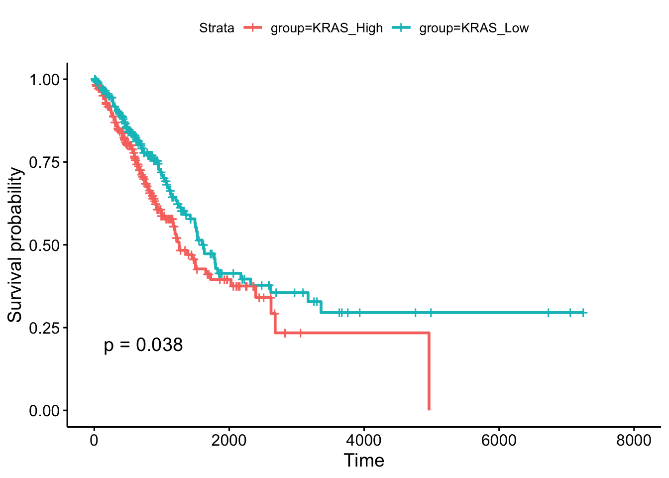 Figure 2. Kaplan-Meier curve. Survival probability vs Time (days)
The Kaplan-Meier plot shows what percent of patients are alive at a time point. We can clearly see that patients in ‘KRAS_Low’ group have better survival than patients in ‘KRAS_High’ group because the survival probability of ‘KRAS_High’ group is always lower than ‘KRAS_Low’ group over time (the unit is ‘day’ here). The difference between the two groups is statistically significant (p<0.05 by log-rank test).
🔗 Related project
XenaShiny, a Shiny project based on UCSCXenaTools, is under development by my friends and me.
🔗 Acknowledgements
We thank Christine Stawitz and Carl Ganz for their constructive comments. This package is reviewed by rOpenSci at https://github.com/ropensci/software-review/issues/315.
Wang et al., (2019). The UCSCXenaTools R package: a toolkit for accessing genomics data from UCSC Xena platform, from cancer multi-omics to single-cell RNA-seq. Journal of Open Source Software, 4(40), 1627, https://doi.org/10.21105/joss.01627 ↩︎
Filed under
Suggest an edit
Open a pull request
